110110 Differential Equations

The equation

F_net = m a

expresses Newton's Second Law, which relates the acceleration of a mass m to the net force acting on that mass.

Since the acceleration function a(t) is equal to the second derivative x '' (t) of the position function x(t), Newton's Second Law can be written in terms of derivatives as

F_net = m x '' ,

This is always so.

So the equation

m x '' = F_net

is very important in applications.

We will use this equation to understand some basic things about differential equations.

SHM (simple harmonic motion) occurs then F_net = - k x.  In this case our equation becomes

m x '' = - k x.

We rearrange this to the form

x '' = - k / m * x.

To clarify some terminology:

This equation relates a function x(t) to at least one of its derivatives, so we call it a differential equation. 

The highest derivative in this equation is the second derivative.  So we call this a second order differential equation.

An example of a first-order differential equation might be

x ' = t + x.

Note that this equation contains the variable t as well as the function x and its derivative x '.

We could write this equation as

x ' = f(t, x),

where f(t, x) = t + x.

This equation looks very simple, and it isn't all that complicated, but it's harder than it looks.  You are unlikely to be able to find a solution to this equation until we have developed some more terminology to classify equations, and the the machinery to solve this particular type of equation.

An equation we can easily solve is

x ' = t.

Remember that x ' is the derivative of the x(t) function with respect to t.  Thus x(t) is an antiderivative of x ' (t), and if we integrate x ' (t) with respect to t we get x(t).  There is also a constant involved in the integration, but we will take care of that when we integrate the equation.

Integrating both sides of the equation, we therefore get

x (t) = 1/2 t^2 + c,

where c is a constant.  Both sides of the equation would have integration constants, so c represents the integration constant from the right-hand side, minus the constant from the left-hand side.

So x(t) = 1/2 t^2 + c is the general solution to our equation x ' = t.

The integration constant allows us to impose one condition on our solution.  For example if we want to impose an initial condition that x(0) = 12 (we call this an initial condition because it applies at t = 0), we can accomodate that:

x(t) = 1/2 t^2 + c so

x(0) = 1/2 * 0^2 + c = c.

Thus, if x(0) = 12, we have

12 = c.

Our specific solution (called a particular solution) to the equation is therefore

x(t) = 1/2 t^2 + 12.

If x(t) represents the position function for a particle with constant acceleration a, then the fact that acceleration is the second derivative of the position leads us to the equation

x '' (t) = a = constant.

An antiderivative of x '' (t) is x ' (t), and an antiderivative of the constant quantity a is a t.  So a single integration of our equation yields

x ' (t) = a t + c_1,

where c_1 is a constant number.

Integrating once more we get

x(t) = a * t^2 / 2 + c_1 * t + c_2,

where c_1 is the integration constant from our previous integration and c_2 is the constant from our present integration.

The two constants allow us to impose two conditions on our solution.  For example we could impose the conditions x ' (0) = 5 and x(0) = 7.  In terms of motion, x ' represents velocity and x represents position, so our conditions specify an initial velocity and an initial position on our motion.

The first of our integrals is x ' (t) = a t + c_1.  You can verify that the condition x ' (0) = 5 gives us c_1 = 5.

Our position function is therefore x(t) = a t^2 / 2 + 5 t + c_2.  You can verify that our condition x(0) = 7 gives us c_2 = 7 so that our position function becomes

x(t) = 1/2 a t^2 + 5 t + 7.

In general if x(0) = x_0 and v(0) = x ' (0) = v_0, our general solution x(t) = a * t^2 / 2 + c_1 * t + c_2 becomes

x(t) = 1/2 a t^2 + v_0 t + x_0.

You should recognize this as a standard equation of uniformly accelerated motion in introductory physics.

In general a first-order differential equation will yield one arbitrary constant, allowing us to impose one condition on the solution, and a second-order equation will yield two arbitrary constants, allowing us to impose two conditions. 

If an equation is of order n, then a general solution will include n arbitrary constants, allowing us to impose n conditions on our solution.

Returning to the equation for SHM:

x '' = - k / m * x,

we don't yet have a method for solving this equation.  There is a simple method (let x = A e^(r t) and see what this tells us about the two arbitrary constants A and r).  You might have seen this method in your first-year calculus course, which often includes a brief introduction to differential equations.  The method is not difficult, and we will see it in a later chapter.

Here we simply assert that the general solution to the equation can be expressed as

x(t) = B cos( sqrt(k/m) t ) + C sin ( sqrt(k/m) t ).

If you plug this function into the equation x '' = -k/m x, you can easily verify that x '' (t) is in fact equal to -k /m * x(t).

As expected, this solution includes two arbitrary constants B and C.

Basic trigonometric identities allow us to rearrange the expression B cos( sqrt(k/m) t ) + C sin ( sqrt(k/m) t ) into the expression A cos( sqrt(k/m) t + phi ), where A and phi are constants that can be expressed in terms of B and C in the original form.  So another way of writing the solution is

x(t) = A cos( sqrt(k/m) t + phi).

You should verify that this is also a solution of the equation.

Both solutions can be written in terms of omega = sqrt(k /m):

x(t) = B cos( omega * t) + C sin( omega * t)

x(t) = A cos(omega * t + phi) ).

The second solution is easily interpreted as the x component of a position vector r ( t ) whose terminal point moves with angular velocity omega around a circle of radius A, with initial angular position phi.

x(t) is therefore the general equation of motion for a simple harmonic oscillator with amplitude A and angular frequency omega = sqrt(k / m).

You should verify that x(t) = A cos(omega * t + phi), with omega = sqrt(k/m), is a solution of the equation x '' = -k / m * x.

An object moving against a constant frictional force F_frict and an air resistance - k v which is proportional to its speed has

F_net = -F_frict - c v, so that

m x '' = -F_frict - c v and

x '' = -F_frict / m - c / m * v.

Since v = x ' this equation becomes

x '' = -F_frict / m - c / m * x '.

We won't at this point discuss how to classify or solve this equation.  However note the following:

This is a second-order equation, with x '' expressed in terms of t, x, and x '.

In fact x '' is expressed only in terms of x ', with no specified dependence on t or x. 

The equation is certainly of the form

x '' = f(t, x, x '),

though in this case t and x aren't actually part of the definition of the function f.

If the object in the preceding is also subject to a linear restoring force F = - k x (e.g., consider a mass oscillating on a smooth tabletop while attached to a spring; friction and air resistance are still present but now we have the restoring force of the spring to consider), the equation would be

x '' = -F_frict / m - c / m * x ' - k x.

This is still of the form

x '' = f(t, x, x').

In this case the function f(t, x, x') includes the expressions x and x ', but there is no t dependence.

Now suppose the table is gradually tilted.  The gravitational force on the mass will then have a component parallel to the object's motion, which will increase in magnitude as the table gets steeper.  The equation of motion could then be of the form

x '' = -F_frict / m - c / m * x ' - k x + m g cos ( b t ),

where g is the acceleration of gravity and b is a constant which determines how quickly the angle of the incline changes.

This equation is also of the form

x '' = f(t, x, x ' ),

where now all three of the quantities t, x and x ' are included in the expression for t.

[Physics students may note that the frictional force will no longer be constant when as table is tilted through different angles, so F_frict also becomes a function of t.  This was not mentioned before for fear of overly complicating the equation, but the equation would be x '' = - mu g sin( b t) - c / m * x ' - k x + m g cos(b t).  This is still of the form x '' = f(t, x, x').]

[Instructor note:  Off the top of my head it doesn't appear that the two equations given here have a closed-form solution.  Most differential equations don't.  However we can always generate approximate solutions, and we can often solve a similar equation in closed form and then using reasonable approximations consider how solutions to our actual equation will differ.]

Let's return to the equation x ' = x + t.  This equation can be solved, and we'll soon learn how to solve it.  But unless you've studied differential equations to some extent, you probably can't solve it right now.  So we can pretend that it's just not solvable.

However we can develop an approximate solution.

First note that the equation is of first order, so we can impose one condition on the equation.  Let's say that our condition is that x = .37 when t = .30.

We can reason as follows:

If x = .37 and t = .30, then x ' = x + t = .37 + .30 = .67.

x ' tells us how quickly x changes with respect to t, so that as long as x ' doesn't change too significantly,

`dx = x ' * `dt

is a good approximation to how much x will change as a result of a change in t.

Without a lot of further analysis, let's just see what happens if we assume that a change `dt = .1 doesn't significantly affect the value of x '.  This might or might not be the case, depending on your interpretation of the word 'significant' for the specific situation.

Now, if x ' = .67, then `dt = .1 gives us a slope of .67 and a 'run' of .1, which will result in a 'rise' equal to slope * run =  .67 * .1 = .067.

Remember that we started with x = .37.  Adding a 'run' of .067 we end up with x = .37 + .067 = .437.

An interval `dt = .1 increases the value of t from .30 to .40.

The approximate value of x, expected at t = .40, is therefore .437.

We can summarize the same series of calculations more formally as follows:

Our equation is x ' = f(t, x) = x + t.

At (t, x) = (.30, .37) we have x ' = f( .30, .37) = .67.

Using `dt = .1, our approximation for the change in x is

`dx = x ' * `dt = .67 * .1 = .067.

Our approximation is therefore

(t_new, x_new) = (30 + .1, .37 + .067) = (.40, .437).

There is no need to stop at this point, except to note that between our original point and our new point, x ' will indeed change.  Remember that we did assume that x ' didn't change significantly.  When x = .437 and t = .40, our value of x ' will be x ' = x + t = .837.  Comparing this with .67, we see that there is about a 20% difference, and our estimate of `dx is probably off by about 10%.  Depending on what we're trying to accomplish with our solution, this might or might not be significant.  Taking into account other uncertainties in our situation we might decide that we need to do better.  It would be easy to do so by reducing our `dt.  For example, reducing `dt to .01 would result in the approximate point (.3767, .31), at which x ' would be .6867.  We would expect our approximation to be off by only about 1%.  The disadvantage is that we would not yet have a value of x corresponding to t = .40.  Another option, based on `dt = .1, would be to average our two values .67 and .837 of x ', and use this average to recalculate our new x value.

In any case, continuing our original approximation, we can use our new point (.437, .40) to predict a new point:

Our equation is x ' = f(t, x) = x + t.

At (t, x) = (.40, .437) we have x ' = f( .40 , .437) = .837.

Using `dt = .1, our approximation is for the change in x is

`dx = x ' * `dt = .837 * .1 = .084,

where we have rounded off our `dx to two significant figures (more significant figures would be meaningless because of the error inherent in the approximation process).

Our new approximation is therefore

(t_new, x_new) = (.40 + .1, .437 + .084) = (.50, .53),

where again we have rounded to 2 significant figures.

We now have three points:  (.37, .30), (.437, .40) and (.50, .53).

If you plot these points on a graph of x vs. t, you will see that they indicate a curve which is concave upward.  This is what we would expect based on our calculations, since according to our calculations the values of x ' are positive and increasing (positive x ' means a positive slope, increasing x ' means increasing slope).

This curve is an approximate solution curve for our function. 

Our curve is only approximate, since it is based on the assumption that x ' doesn't change between points.

Approximation errors accumulate with every step, multiplying in such a way that our curve varies more and more from the actual curve.

We could get a better approximation to the curve by using a smaller increment `dt (e.g., `dt = .01).  It would take us 20 steps instead of 2 steps to get to the t = .50 point, but we would end up with a much more accurate solution curve.

Or after our first approximation of the new point, we could calculate the slope at the new point then re-predict that point based on the average of our two slopes.  Using this method with `dt = .1 would give us a far more accurate solution curve in fewer steps than would be required with `dt = .01.  There would be about twice as much calculation per step, but we would still be ahead.

Another way of analyzing solution curves is to use direction fields. 

For any point (t, x) of the x vs. t plane, the equation x ' = x + t can be evaluated to obtain a value of the slope x '.  Through any such point we can sketch a short line segment of the corresponding slope, and this segment will be the slope of a solution curve through that point.

If we do this for a grid of points, we get a direction field.

For the equation x ' = x + t, it is easy to evaluate x ' for the points on the grid

(0, 0), (0, 1/4), (0, 1/2), (0, 3/4), (0, 1)

(1/4, 0), (1/4, 1/4), (1/4, 1/2), (1/4, 3/4), (1/4, 1)

(1/2, 0), (1/2, 1/4), (1/2, 1/2), (1/2, 3/4), (1/2, 1)

(3/4, 0), (3/4, 1/4), (3/4, 1/2), (3/4, 3/4), (3/4, 1)

(1, 0), (1, 1/4), (1, 1/2), (1, 3/4), (1, 1).

The respective slopes range from 0 to 2.  The respective slopes are

0, 1/4, 1/2, 3/4, 1

1/4, 1/2, 3/4, 1, 5/4

1/2, 3/4, 1, 5/4, 3/2

3/4, 1, 5/4, 3/2, 7/4

1, 5/4, 3/2, 7/4, 2

Plotted on a graph of x vs. t, we get something like the picture below:

All we have done is evaluate our function f(x, t) at a number of points within our region of interest.

It's easy to make a similar plot for any function f(x, t).  All we need to do is plug in x and t values.

Having plotted our direction field, we can then sketch a solution curve starting from any point in the field.

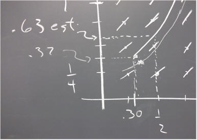
The curve through (.30, .37) is approximated based on the hand-sketched direction field.

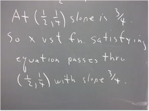
The t = .5 value of x predicted by the hand-sketched curve on the hand-sketched direction field is .63.  Our calculated prediction was x = .53, and our approximations were seen to underestimate the actual changes in x, so a prediction of .63 might not be bad.  However our calculated predication of the total change in x (which is .53 - .37 = .16) is probably not off by much more than 20%, and the sketch predicts a change of .63 - .37 = .26, so we can't claim a lot of accuracy for the hand sketch.  The main value of the hand sketch is to provide a geometric picture of the behavior of this differential equation.

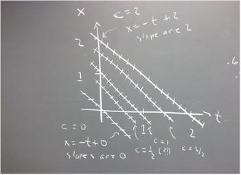
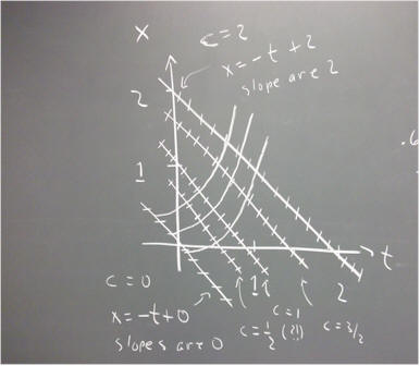
Direction fields are easy enough to sketch using a grid (though of course the process could be tedious).  The process becomes much easier if we use isoclines:

f(x, t) = x + t has constant value c when x + t = c.

x + t = c when x = -t + c.

x = -t + c describes a straight line in the x vs. t plane, with slope -1 and y-intercept c.

It's easy to sketch these lines for a set of c values.

For c = 0, 1/2, 1, 3/2, 2 our lines would look something like the ones in the picture below:

The slope corresponding to each value of c is equal to c (this since x + t = c, and the slope is x ' = x + t).  A number of segments of more or less appropriate slope have been sketched along each line.  All the slopes along each line are the same, which makes it fairly easy to draw a decent slope field.

The figure isn't very well drawn; for example the c = 1/2 and c = 3/2 lines are badly misplaced, and the c = 1 line clearly missed the point (1, 0) on the t axis.  The artist blames an unbuttoned sleeve for blocking his vision.  Use of a straightedge and more care would have also been helpful.

The figure below depicts three solution curves.  A solution curve can be sketched starting at any point, and moving either to the right or to the left.  Once the slope field is drawn, the solution curves are fairly easy to sketch.

Had the equation been x ' = x + t^2 instead of x + t, the constant-slope condition would have been x + t^2 = c.  This would give us x = -t^2 + c, which for each value of c is a parabola rather than a straight line. 

In general, the equation x ' = f(x, t) yields constant-slope curves f(x, t) = c. 

f(x, t) = x + t gives us a series of straight lines, along each of which the slope is constant.

f(x, t) = x + t^2 gives us a series of parabolas, along each of which the slope is constant.

In general a function f(x, t) gives us a series of curves f(x, t) = c, along each of which the slope is constant.

These curves are called isoclines ('iso' for 'one', 'cline' for inclination).

Spreadsheets and computer programs have obvious applications to the calculation schemes we have introduced here.

Let's consider for a moment the case of a second-order equation of the form

x '' = f(x, x', t).

We can still imagine a geometric picture depicting the behavior of the function f(x, x' t).  However our picture graph would be in 3 dimensions, with an axis for each quantity x, x ' and t.  Values of x '' would dictate changes in x ', not it x; and changes in x ' would then dictate changes in x.  Our solution curves would become surfaces in a 3-dimensional space, our 3-dimensional space would no longer represent the 3-dimensional space we live in, and x vs. t solution curves would represent the intersections of these surfaces with the planes x ' = constant.

It's even more fun to try to imagine what happens when we go into higher dimensions.

However the scheme for numerically approximating the solution curves of a second-order equation isn't that much more complicated than the scheme we saw here.