Combining Functions Graphically

Class Notes Precalculus I, 12/02/98

Combining Functions Graphically

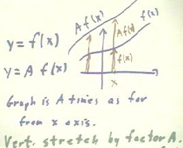
Given the graph of y = f(x), we obtain the graph of y = A f(x) by multiplying each y value of original graph by A.

In the figure below, we see that we can perform this operation for a single value of x by picking a point (x,0) on the x axis and sketching a vector from the point to the graph of f(x).
The length of this vector represents the value y = f(x).
If we then multiply the length of this vector by A, we obtain a vector from the x axis to the graph of y = A f(x).
This vector is shown for A approximately equal to 2.

We can then repeat the process for another value of x, as depicted below.

We can repeat the process for as many values of x as necessary to determine the shape of the graph of the function y = A f(x).

At every x, we will 'stretch' the vector representing f(x) by the factor A.
We therefore say that this transformation constitutes a vertical stretch of the graph of y = f(x) by factor A.

We have previously seen this process of vertical stretching illustrated in detail for the y = x² function.

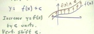
We can contrast vertical stretching with the vertical shifting that results from the transformation y = f(x) + c.

This transformation increases the value of y at each point by the amount c.
Graphically this corresponds to raising every point of the graph of y = f(x) by c units.
This is represented below by vectors of length c from points of the f(x) graph to points of the graph of f(x) + c.

We have previously seen this shifting process illustrated for the function y = x ².

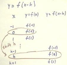
We have also seen the shifting behavior that relates the graph of y = x² to that of y = (x-h)².

Recall that

for y = x² the values y = 9, 4, 1, 0, 1, 4, 9 occur at x = -3, -2, -1, 0, 1, 2, 3, whereas

for y = (x-h)², y = 0 occurs for x = h and the values 9, 4, 1, 0, 1, 4, 9 occur for x = h-3, h-2, h-1, h, h+1, h+2 and h+3.

The result is that the graph of y = x² is shifted h units in the x direction.

The graph of y = f(x-h) is in general related to the graph of y = f(x) in a similar manner.

At x = 0, y = f(x) takes value f(0), whereas the function y = f(x-h) takes the same value f(0) at x = h.
We see this illustrated on the table below. In this figure the points where y = f(0) are circled in red.
We see that the x coordinate of the point where y = f(0) is shifted h units.

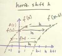
As illustrated on the table below, at x = -1, 0 and 1, the function y = f(x) takes values f(-1), f(0) and f(1), whereas the function f(x-h) takes these values at x = h-1, h and h+1.

The result of these observations is illustrated on the graph below.

At x = -1, 0 and 1, we have plotted points corresponding to arbitrary assumed values for y = f(-1), f(0) and f(1).
The dotted red line indicates the corresponding graph of the assumed function y = f(x).
At the points x = h-1, h and h+1, we have again used two y values f(-1), f(0) and f(1), obtaining points on the 'green' graph of f(x-1).
The graph of f(x-h) will therefore have a similar shape around these points as the graph of y = f(x) around the three 'red' points.
The graph of this function is therefore identical in shape to that of y = f(x), but is shifted h units in the x direction.

Video File #04

http://youtu.be/hOeSUPDqX48

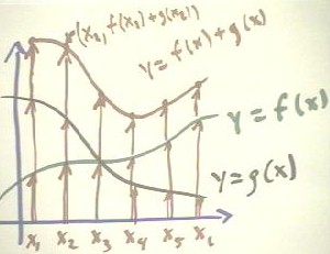
We now consider how to graphically add the functions y = f(x) and y = g(x) shown below.

At x₁, we have sketched a vector from the x axis to the graph of y = f(x), and another vector from the x axis to the graph of y = g(x).
We have then taken a copy of the first vector, representing f(x₁), and placed it tail-to-head with the vector representing g(x₁).
The y coordinate of the tip of the copy of the f(x₁) vector therefore represents f(x₁) + g(x₁) and lies on the graph of y = f(x) + g(x).

We have repeated this process for x = x₁, x₃, ..., x₆, in each case taking the shorter vector and placing it 'on top' of the longer vector to obtain the f(x) + g(x) vector.

Subtraction would follow a similar pattern, but for the function f(x) - g(x), for example, we would turn the g(x) vector 'upside down' before placing it head-to-tail with the f(x) vector.

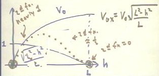
We now consider the process of multiplying two functions.

Recall that for the example of the ball rolling down the incline then falling to the floor, the initial velocity v_0x in the x direction was obtained by multiplying the velocity v0 of the ball by the proportionality factor `sqrt(L² - h²) / L.

As the ramp is raised, with the altitude h of the higher and above the table therefore increasing, the speed v0 of the ball as it leaves the ramp increases.
This speed starts out at 0, for a level ramp with h = 0, and increases at first rapidly with increasing h.
Then as h approaches the length L of the ramp, at which point the ramp will become vertical, the speed of the ball more and more gradually approaches the 'straight-drop' speed of the vertical ramp.
This behavior of v0 is illustrated by the graph of v0 in the figure below.

The proportionality `sqrt(L² - h²) / L, which tells us how much of the initial velocity v0 is in the x direction, has a graph something like that depicted in the figure below.

When h = 0, `sqrt(L² - h²) / L = `sqrt(L² - 0) / L = L / L = 1.

By the time h = L, `sqrt(L² - h²) / L = `sqrt(L² - L²) / L = 0.

So the graph falls from y = 1 to y = 0 as x goes from 0 to 1.

The graph as sketched is not very accurate, though it does fall from 0 to 1. The actual graph will start out horizontal, and will fall much more sharply near the end, approaching vertical as x -> L.

Video File #05

http://youtu.be/2B_cUXzEpNg

Since the velocity v_0x we are seeking is found by multiplying v0 by the factor `sqrt(L² - h²) / L, we can obtain a graph of v_0x vs. x by multiplying the graphs of the two functions.

This means that for every point on the h axis, we multiply the corresponding y values of the two functions.

We see immediately that when h = 0, v0 = 0, so the product of the two functions will be 0.

Furthermore, when h = L, `sqrt(L² - h²) / L = 0, and the product of the two functions will again be zero.

We have indicated the zeros by the large red circles on the h axis.

These points will be the zeros of the product function.

When h is near 0, `sqrt(L² - h²) / L will be near 1, but as h moves away from 0 the function will fall gradually below this value.
So when we multiply the values of this function by v0, we will obtain values near 1 * v0, but falling gradually below this value as h moves away from 0.
So for the first 1/4 of the graph or so, we will have the behavior indicated by the red dots, staying close to the graph of v0 but falling gradually below it.

By the time we get to the point where `sqrt(L²-h²)/L is 1/2, as indicated on the graph by the note '2d fn. = 1/2', the product of the functions will clearly be 1/2 v0, and the graph will be half as high as the v0 graph.

So the graph will have to turn more and more rapidly away from the 'near v0' behavior it started with in order to reach the 'half-as-high' point. Then the graph will continue decreasing toward the zero at h = L.

The resulting 'red' point graph shows us how the initial x velocity v_0x, obtained by multiplying the graph of v0 vs. h by the graph of `sqrt(l²-h²)/L vs. h, changes as the ramp is raised.

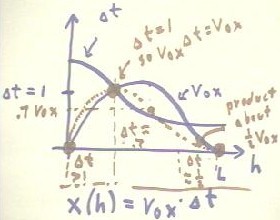
We can further illustrate the behavior of the ball.

Recall that the x range of the ball increased as the ramp was raised above the table, increasing more and more gradually until a maximum range was reached, then decreasing to zero.
Recall also that the x range was the product x = v_0x * `dt of velocity and the time required to fall.
We can therefore get a graph of x vs. h by multiplying the graphs of v_0x vs. h and `dt vs. h.

We begin by sketching the graph just obtained for v_0x vs. h, indicated on the figure below.

We then sketch a graph of `dt vs. h, noting that as h increases the ball has a greater and greater downward velocity as it leaves the ramp and therefore reaches the floor in shorter and shorter times.
The graph shown for `dt below isn't really all that accurate, but it is plausible enough and certainly shows that the time `dt gets shorter and shorter as h increases.

Since v_0x is 0 at h = 0 and at h = L, the product function will also be zero at these points.

These points are indicated by the large red dots on the h axis.

We note also that `dt = 1 at the indicated point of the y axis, so that for our sketch `dt is initially greater than 1.

`dt reaches the value 1 at the indicated point, which is only coincidentally the point where the `dt and v_0x graphs meet.

At the corresponding value of h, we will therefore multiply v_0x by 1, obtaining the point on the v_0x graph.

To the left of this point, `dt is greater than 1, and we will multiply v_0x by a number greater than 1.

The graph of the product function, depicted by the red dots, will therefore remain higher than that of the v_0x graph for this region.

To the right of the point where `dt = 1, we see that `dt gradually decreases, so that we will be multiplying the value of v_0x by numbers less than 1.
Since the product function must approach 0 at h = L, it will therefore decrease in approximately the manner shown.

Near h = L, `dt is approximately 1/2, so the graph of the product function will be approximately half as high as a graph of v_0x.

The graph will therefore approach its zero with a slope about half as great as that of the v_0x function.

The approximate point where `dt = .7 is indicated by a fourth large red dot on the dotted red graph of the product function. At this point v_0x `dt will be approximately .7 v_0x, as indicated on the y axis.

Video File #06

http://youtu.be/IK-EPumvZTs

The resulting function for x = v_0x * `dt has the expected behavior, with the range of the ball increasing from x = 0 to a maximum then decreasing back to x = 0.

To accurately determine the maximum point, we would have to have accurate graphs of v_0x and `dt.
Given such graphs we could combine them in the manner illustrated to obtain an accurate graph of range vs. h.

These examples should illustrate how the concept and the process of multiplication of functions can help illuminate real-world events. They should also illustrate a few important principles to be used in multiplying functions. The basic principles are these:

When one of the functions is zero, the product is 0.
When one of functions has value 1, the product is simply equal to the other function and the corresponding point lies on the graph of that other function.
When one of the functions has a value greater than 1, the product function will have a y value which is correspondingly further from the x axis than the value of the other function.
When one of the functions has a value between 0 and 1, the product function will have a y value which is correspondingly closer to the x axis than the value of the other function.

To these we can add the following:

When one of the functions has a negative value, the product function will have a y value on the side of the x axis opposite of the value of the other function.

We illustrate these ideas by multiplying graphically the functions y = f(x) (in blue, on the graph below) and y = g(x) (in green on the graph below).

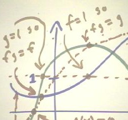
You should look at the graphs of these two functions and note where each function is 0, where each function takes value 1 and where each function takes value -1.

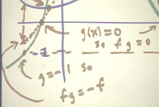
The function y = f(x) is never zero.

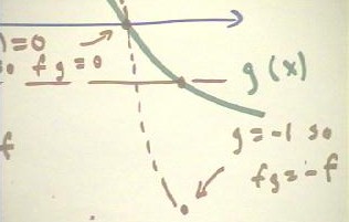
The points where the function g(x) takes value 0 are indicated on the x axis.

The product function must be 0 at these points.

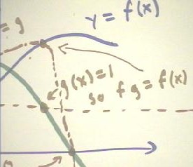
There are two points where g(x) = 1.

You should carefully note the locations of these points and the corresponding points on the graph.

At each such point we note that g = 1 so fg = f, and the point of the graph of fg is therefore on the graph of the f(x) function.

We similarly note the point where f = 1 and the corresponding point on the graph of the product function fg, which coincides with the point on the graph of the g(x) function.

From the points so obtained, we can sketch a reasonable approximation of the graph of f(x) * g(x) between the points where g(x) = 0.

You should trace the red dotted-line graph of f(x) * g(x) through the indicated points.

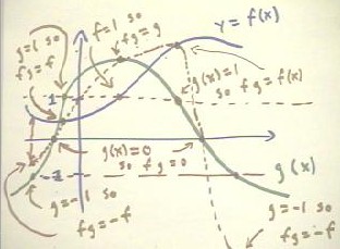
At the left of the graph we note the point where g(x) = -1.

At this point the graph of f * g will take the value -f, opposite to the value on the graph of f(x).

This is indicated by the reversed arrows, with the upward arrow indicating the value of f(x) and the downward arrow indicating the value of f(x) * g(x) = -1 * f(x) = -f(x).

This behavior is also shown in a closeup view on the graph below.

The other point where g(x) = -1 is indicated on the original graph.

Again the graph point for the f * g function will be on the opposite side of the x axis from that of the f(x) function, and will be a 'reflection' of this point.

The graphs below are closeups of important regions of the original graph.

Video File #07

http://youtu.be/TKdcJluU4NA