Class 0826

Depth vs. Clock Time, Initial Model

Make a table of depth vs. clock time, where clock time is the time on an imaginary clock that started at t = 0 at the instant of the first reading.

Sketch a graph of depth vs. clock time, given that with every reading depth decreased by 10 cm.

Conventions:  independent variable vs. dependent variable.  When graphing, the dependent variable goes on vertical or 'y' axis and independent vbl on the horizontal or 'x' axis.  When making a table the independent vbl goes in the first column, the dependent in the second.

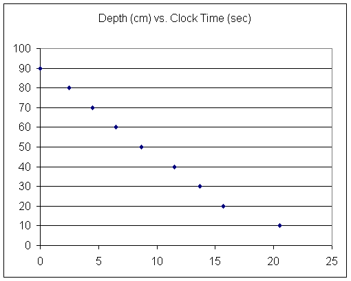
With the depth vs. clock time data taken in class we get the following graph:

Note that there was considerable inconsistency between results obtained for the same trial by different observers. 

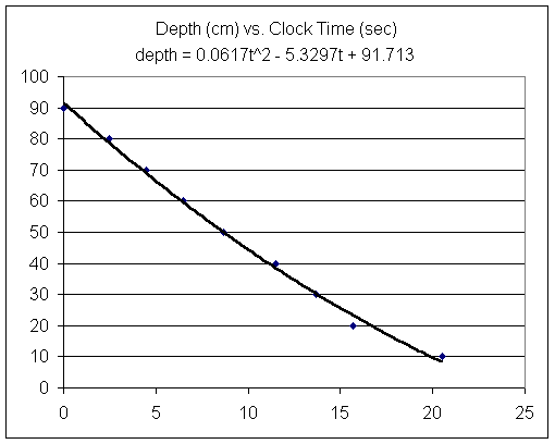
For reasons we'll be able to analyze later in the course this situation should theoretically be modeled by a depth function which is quadratic in time.  So we fit our data with a second-degree polynomial.

As indicated on the graph the equation of the best-fit quadratic function is

• depth = 0.0617t^2 - 5.3297t + 91.713

What was depth at t = 0, 5, 10, 15, 20 sec?

• Plugging in t = 0, 5, 10, 15, 20 we get the following depth vs. clock time table.

• 0	91.713
  5	66.607
  10	44.586
  15	25.65
  20	9.799
  25	-2.967

At what instant was depth 0?

• Using the quadratic formula we get depth = 0 when 

0.0617t^2 - 5.3297t + 91.713 = 0, or when 

t = 62.65783445 or t = 23.72304074.

• We reject t = 62.7 sec for this situation because once the depth first reaches 0, which happens at t = 23.7 sec approx., it keeps going down and doesn't increase again.

At what instant was depth 60 cm?

• To find when depth = 60 cm we set the depth function equal to 60 cm.  This gives us

0.0617t^2 - 5.3297t + 91.713 = 60.

• We put this equation into the form at^2 + bt + c = 0 by subtracting 60 from both sides.  We get

0.0617t^2 - 5.3297t + 31.713 = 0

• We get solutions t = 6.428679398 or  t = 79.95219580.
• We reject the second solution for this situation (again depth goes down and never comes back up) and conclude that depth is 60 cm at t = 6.4 sec.

At what instant was depth 30 cm?

• Using similar strategy we get t = 13.8 sec.

At what average rate does this function indicate the depth is changing between t = 0 and t = 5? 

• During this time interval the depth changes from 91.7 cm to 66.6 cm, a change of 66.6 cm - 91.7 cm = -25.1 cm.
• The average rate of depth change from 0 to 5 sec is -25.1 cm / (5 sec) = -5.02 cm/s.

Answer the same question from the intervals from t = 5 to t = 10, from t = 10 to t = 15, etc.

• The rates are respectively

• -5.0212

  -4.4042

  -3.7872

  -3.1702

  -2.5532

If we assign the average rate to the midpoint time of the interval we get

For homework, graph ave rate vs. midpt clock time and see what is the nature of that graph.  Try to get an equation for that graph.