Calculus 1 Quiz 0909
The derivative of a t^3 + b t^2 + c t + d is 3 a t^2 + 2 b t + c.
y ' (30) = -52
y ' (60) = -85
Average of the two rates is ave of two rates = (y ' (30) + y ' (60) ) / 2 = -68.5
Note that this is not necessarily the average rate (almost certainly won't be unless rate fn is linear)
`dy = ave rate * `dt, which is approximately equal to ave of rates * `dt.
Our approximation is therefore -68.5 * ( 60 - 30) = -68.5 * 30 = -2055
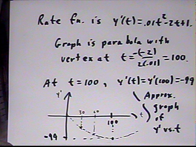
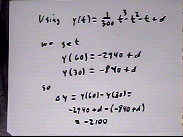
y ' (t) = .01 t^2 - 2 t - 1 so we have 3 a = .01, 2 b = - 2, c = -1 in the form y(t) = a t^3 + b t^2 + c t + d so a = .0033..., b = -1 and c = -1 giving us y(t) = .0033... t^3 - t^2 - t + d. The parameter d is unknown.
Actual change is `dy = y(60) - y(30). Due to the nonlinearity of y ' (t) function this is not exactly equal to the change predicted on the basis of the initial and final rates.
y(60) = d - 2940 and y(30) = d - 840 so
They're different because the rate function is nonlinear.
For the rate function y ' (t) = .01 t^2 - 2 t - 1 of the quiz, approximately what would you expect the change in depth to be for an interval of .1 at t = 60? Recall that y ' (60) = -85.
Interpreting in units of cm and sec, we have rate -85 cm/s and time interval .1 sec. At -85 cm/s in `dt = .1 sec the change would be -85 cm/s * .1 sec = -8.5 cm.
Is this an exact estimate? If not how close is it?
It's not exact. The rate function will change during the .1 sec interval. But it won't change much so we've got a very accurate, if not perfect, estimate.
The quiz problem is analyzed once more.
Graphing the rate function (vertex at t = -b / 2a = 100, so y = y(100) = -99) we see that it is concave up between t = 30 and t = 60.
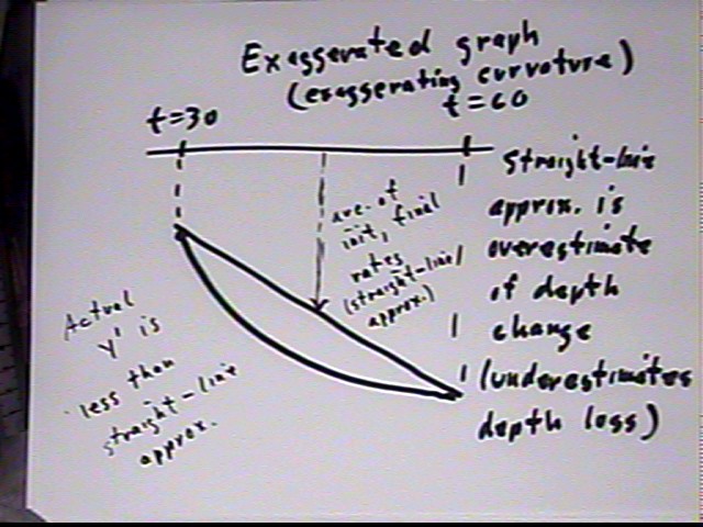
Exaggerating the curvature of the graph we see why the process of averaging initial and final rates, which is equivalent to using a straight-line approximation to the rate function, to approximate the average rate will overestimate the depth change (and hence underestimate the loss in depth).
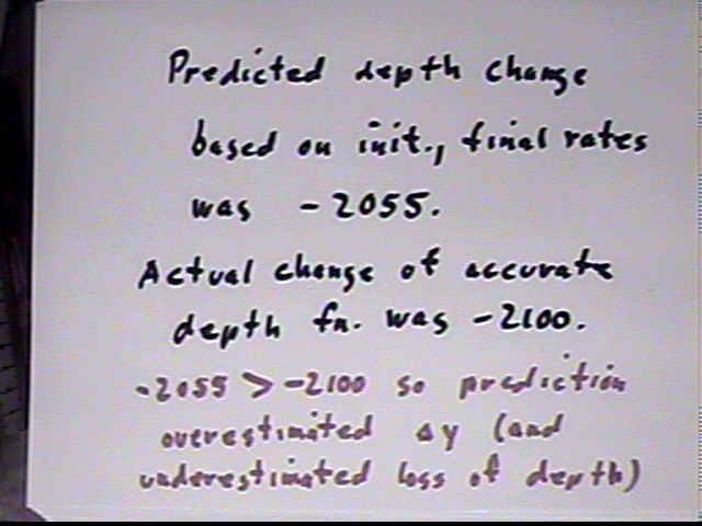
The accurate depth change is based on the y(t) funciton. We get depth change = -2055.
Our prediction based on initial and final rates was -2055.
Since -2055 > -2100 our estimate was greater than the actual change, confirming our conclusion that for this rate function the linear approximation overestimates the change and underestimates the loss of depth:
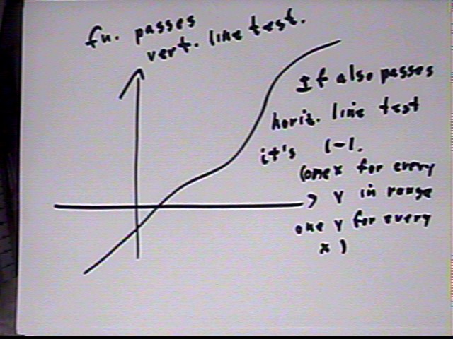
A function must pass the vertical line test. If it also passes the horizontal line test then the function is 1-1, meaning that for every number in its domain there is exactly one number in its range:
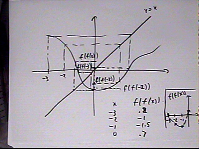
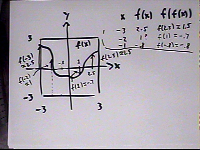
Given a graph of f(x) we can do point-by-point estimates to get an approximate table for f(f(x)), from which we could construct a graph of f(f(x)).
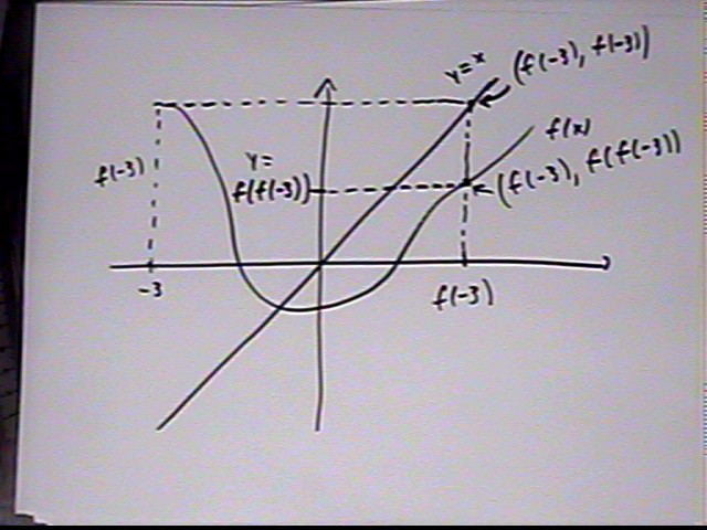
We can also use projections and the line y = x to obtain estimates (note that the function as drawn here is a little different from the function used for the preceding estimates so the results will be different).
We project from x on the horizontal axis to the graph of the function the horizontally to the line y = x, placing us at the point (f(x), f(x)).
When we project from (f(x), f(x)) vertically to the graph we will be at the point (f(x), f(f(x)).
Projecting horizontally to the y axis we obtain the value f(f(x)).
Following this procedure for x = -3, -2, -1, 0 we arrive at estimates for f(f(x)) at these x values. We construct a table and an approximate graph.