Calculus I Quiz 0918
Given that y ' (t) = -.02 sqrt(y(t)) * (t / 10) and the knowledge that at t = 0 we have y = 100, use an interval `dt = 10 to estimate y(t) at t = 10.
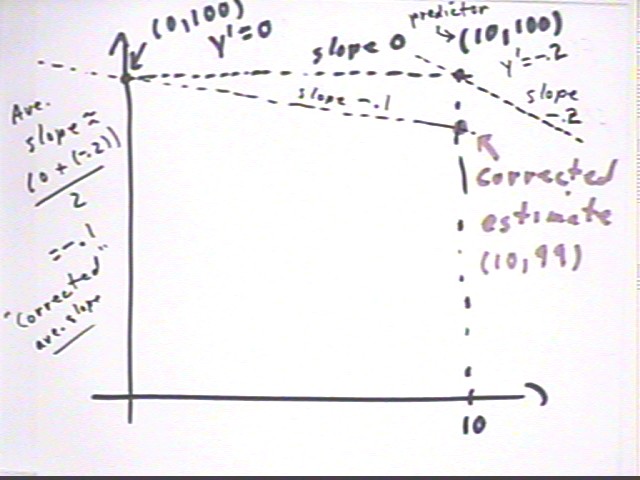
At (0, 100) we have y ' (t) = -.02 sqrt(100) * 0 / 10 = 0.
Using y ' = 0 we get `dy = y ' `dt = 0 * 10 = 0.
So the new predicted value of y at t = 10 is 100 + 0 = 100.
Now find y ' at the t = 10 point.
The t=10 point is (10,100) so we get y ' = -.02 * sqrt(100) * 10/10 = -.2.
Average the y ' estimate at the t = 10 point with the y ' obtained at the t = 0 point.
The average of the two slopes is (0 + -.2) / 2 = -.1. This is a reasonable estimate of the actual ave slope over the interval.
Go back to t = 0 and re-estimate the change in y based on your average.
Based on slope y ' = -.1 we have `dy = y ' `dt = -.1 * 10 = -1. Thus at t = 10 we have y = 100 + (-1) = 99.
The figure below shows
y = 99 is our 'corrected' estimate for the t = 10 point of our graph.
Why should this give an improved result over the one we would get based only on the y ' at the t = 0 point?
We're giving equal weight to the slope at the beginning of the interval and the slope at the end of the interval. This gives a big improvement in our accuracy.
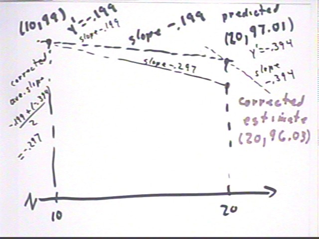
See if you can adapt this improved procedure to obtain an estimate of y at the t = 20 point.
Evaluating y ' at (10,99) we get y ' = -.199 approx.. This would result in `dy = -.199 * 10 = -1.99 and a new y value of 99 + -1.99 = 97.01.
At (20, 97.01) we get y ' = -.394.
We average the slopes -.199 and -.394 at the ends of the interval to get 'corrected' slope -.297.
Using the 'corrected' slope we get y ' = -.297 * 10 = -2.97.
Our 'corrected' value of y is 99 + -2.97 = 96.03.
This process is illustrated below:
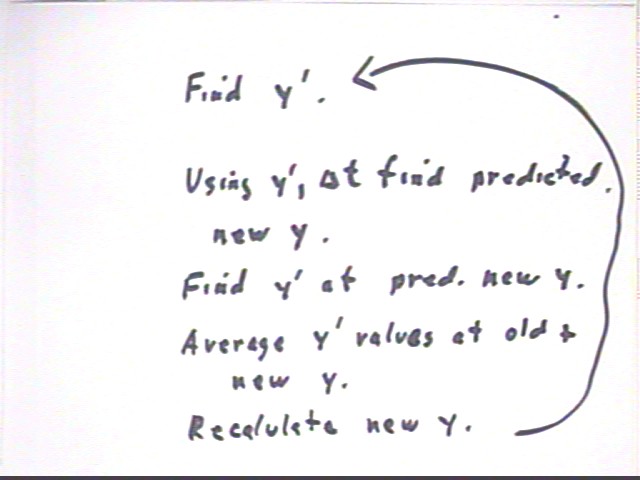
The procedure starts with values of y and t, a desired interval `dt and a rule for calculating y ' . It then proceeds through the following steps, and is then iterated as many times as desired:
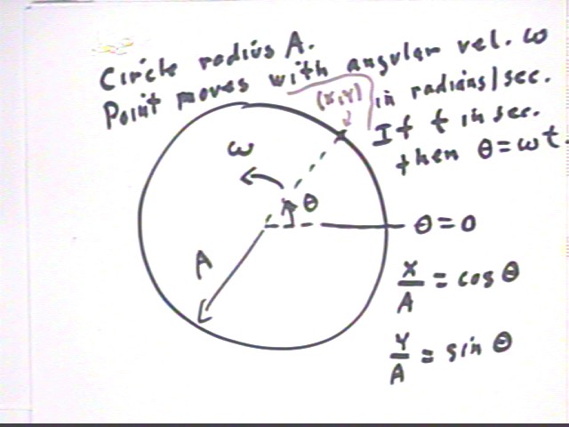
To understand the period and amplitude of the sine and cosine functions we think of a point moving with angular velocity omega, in rad/s, around a circle of radius A.
The angular position at clock time t, starting from the point on the positive x axis, is found by multiplying the number of radians / sec by the number of sec to get the number of radians of angular displacement. So to get the angular position theta we multiply angular velocity omega by clock time t.
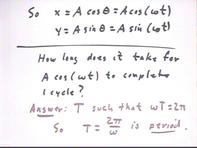
Since x = A cos(theta) = A cos(omega * t), and since the angular position omega * t must change by 2 pi (corresponding to a complete trip around the circle) we see that the time T required for a complete cycle is 2 pi / omega.
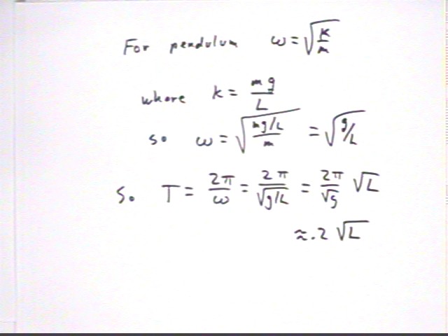
Side note for physics students connecting the formula T = .2 sqrt(L) to this model. The reason for omega = sqrt(k/m) must await full development of the calculus of sine and cosine functions:
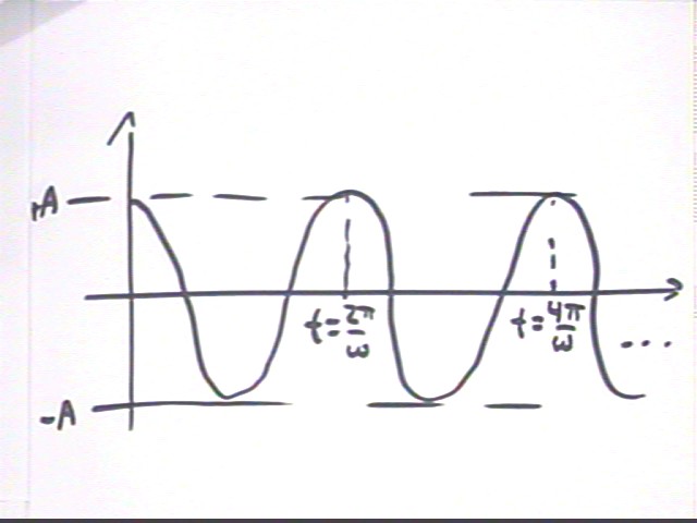
A graph of y = A cos(omega * t) vs. t starts with y = A (since the x coordinate of theta=0 point on ref circle is 1) and moves through y = 0 (the x coordinate at theta = pi/2 is 0) then y = -A, back to y = 0 and finally returning to y = A. The time required for this process is the time required for a complete revolution, 1 period, or 2 pi / omega.
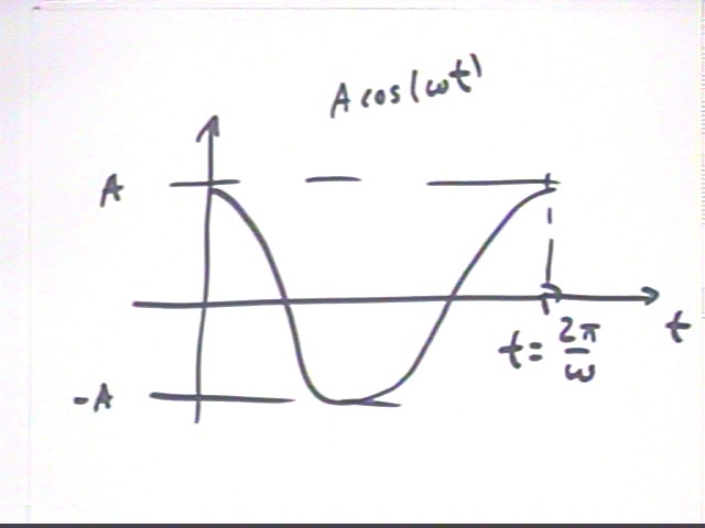
The cosine function passes thru its cycle again and again as the reference point continues to move around the circle, required a time interval of 2 pi / omega for each complete cycle.
The graph below depicts
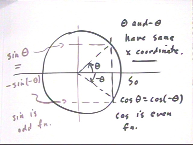
Moving from the theta=0 position through equal angular displacements the positive or the negative direction (counterclockwise or clockwise) we end up with the same x coordinate and opposite y coordinates. This is why the cosine function is odd, the sine function even.
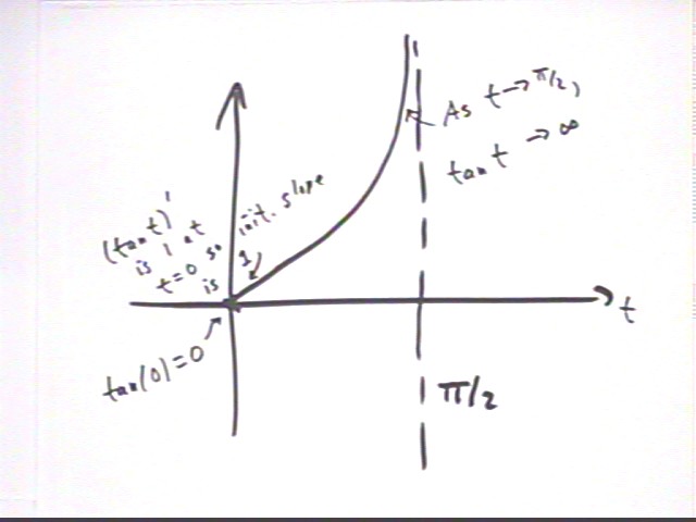
tan(theta) is defined as y / x, which is the same as sin(theta) / cos(theta).
When theta = 0 we have y = 0 and hence tan(0) = 0.
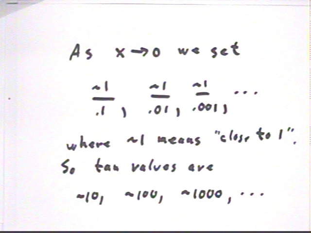
As theta approaches pi/2 we see that y stays close to 1 while x approaches 0, with the result that tan(theta) = y / x approaches infinity.
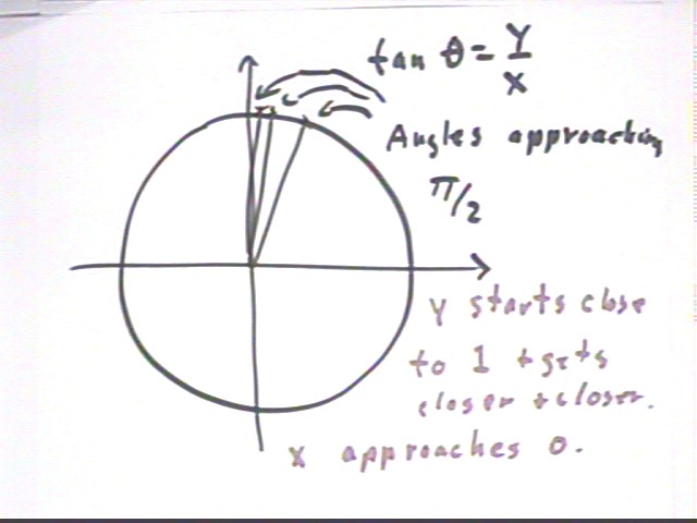
Note that in the figure below ~1 stands for 'close to 1', ~10 for 'close to 10', etc.
The overall shape of the graph of y = tan(t) between t= 0 and t= pi/2 is as depicted below.
The derivative of the tangent function at t = 0 is 1 (we'll see why later) so the graph has slope 1 at the origin.