Calculus I Quiz 0925
Problem: The quadratic depth vs. clock time model corresponding to depths of 80.43184 cm, 72.44526 cm and 68.04026 cm at clock times t = 7.85821, 15.71642 and 23.57463 seconds is depth(t) = .029 t2 + -1.7 t + 92.
The form is quadratic: y = a t^2 + b t + c
Substituting y and t from each data point we get (approx.):
80.4 = a * 7.8^2 + b * 7.8 + c
72.4 = a * 15.7^2 + b*15.7 + c
68.0 = a * 23.6^2 + b * 23.6 + c.
Note that some questions ask you to solve the system to find a, b, c.
rate = depth ' (t) = .058 t - 1.7. At t = 18.4 sec we evaluate depth ' (18.4).
depth(t) = 75 when
.029 t^2 - 1.7 t + 92 = 75.
Solve using Quad Formula
Depth stops changing when rate of depth change is 0, i.e., when
depth ' (t) = 0 or
.058 t - 1.7 = 0
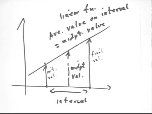
Problem: The depth vs. clock time function y = .029 t2 + -1.2 t + 81 indicates the depth y of water in a certain uniform cylinder at clock time t.
Ave rate of depth change is
change in depth / change in clock time = [ depth(11.6) - depth(5.8) ] / (11.6 - 5.8),
Midpoint t is (5.8 + 11.6) / 2 = 8.7.
Rate at this instant is depth ' (8.7) = .058 * 8.7 - 1.7 = ... .
This result will be identical to the ave rate of change over the interval, since the rate function is linear.
Problem: If the rate of depth change is given by dy/dt = .288 t + -1.8 represents the rate at which depth is changing at clock time t, then how much depth change will there be between clock times t = 5.8 and t = 11.6?
From basic idea of rate:
Depth change = ave rate of depth change * `dt
We're given the rate function. We find the approximate average rate by averaging the initial and final rates on the interval.
Initial rate = .288 * 5.8 - 1.8 = -.13 approx.
Final rate = .288 * 11.6 - 1.8 = 1.54 approx.
So ave rate is (-.13 + 1.54) / 2 = .7 approx.
Thus change in y is
`dy = ave rate * `dt = .7 * (11.6 - 5.8) = 4.06.
If dy/dt = .288 t - 1.8 then y = a t^2 + b t + c where 2 a = .288 and b = -1.8. Thus we have
y(t) = .144 t^2 - 1.8 t + c.
Since y (0) = 220 we have
y(0) = c = 220,
so that c = 220 and
y(t) = .144 t^2 - 1.8 t + 220.
We're given the function to find the values of the quantity at the two clock times. The average rate is change in quantity / change in clock time.
COMMON ERROR: Thinkin' that you have two rates. You ain't given the rates. If you were you would average them to find the approximate average rate, which you could then multiply by the time interval to get approx. change in quantity. But that's not what you got here.
ave rate = `dI / `dt = -0.004253381490 / .1 = -0.04253381490.
At what average rate is the illumination from the lamp changing between clock times t = 17.7 and t = 17.71 seconds?ave rate = `dI / `dt = -0.0004281125337 / .01 = -0.04281125337.
At what average rate is the illumination from the lamp changing between clock times t = 17.7 and t = 17.701 seconds?We find I(17.701) and I(17.7) and subtract to get `dI = - -.00004283917415. We see that `dt = 17.701 - 17.7 = .001. Thus
ave rate = `dI / `dt = -.00004283917415 / .001 = -.04283917415
Looks like it'll be -.0428 something. Probably not far from -.04284.
The figure below illustrates calculation of the average rate between 17.7 and 17.8, then more accurately between 17.7 and 17.71 corresponding to the two slope lines drawn. The result for the interval between 17.7 and 17.701 is indicated, though the line segment and slope triangle are too small to be depicted here.
We can see how the slopes of the line segments must approach the slope of the tangent line.
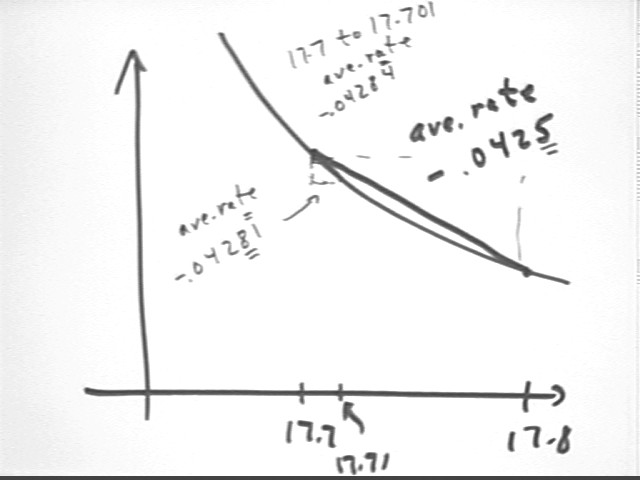
If we calculate the derivative of the function and evaluate it at 17.7 we get -0.04284227851 to 10 sig figures, consistent with the trend of our approximations.
Problem: The rate at which the illumination a newspaper changes is given by Rate = 750 / (t+3)3, where Rate is rate of change in watts/m2 per second and t is clock time in seconds. How much do you think illumination will change between t = 17.7 and t = 35.4 seconds?
Now we're given the rate function. We evaluate the rate function at the two clock times and average the two to get approx. average rate (not a great approximation here because of a fairly long time interval and a nonlinear rate function). Then multiply approx. ave rate by `dt.
Quick Summary:
Ave rate of change of y with respect to t is change in y / change in t.
If y is a function y(t) of t then ave rate of change between t and t + `dt is [ y(t+`dt) - y(t) ] / `dt.
Ave rate of change of y with respect to t between two graph points is represented by the ave slope of the graph between those points, which is equal to rise / run where rise = change in y and run = change in t.
The derivative y ' (t) is the limiting value of [ y(t+`dt) - y(t) ] / `dt as `dt -> 0, and is the instantaneous rate at which y changes with respect to t.
For y(t) = a t^2 + b t + c, the expression [ y(t+`dt) - y(t) ] / `dt simplifies to and expression which as `dt -> 0 approaches 2 a t + b; so we say that y ' (t) = 2 a t + b.
For y(t) = a t^3, the expression [ y(t+`dt) - y(t) ] / `dt simplifies to and expression which as `dt -> 0 approaches 3 a t^2; so we say that y ' (t) = 3 a t^2.
The y ' (t) function corresponding to a given y(t) is the 'rate-of-change function' and is called the derivative function.
The change `dy in the value taken by y(t) near a given t is approximately equal to y ' (t) * `dt .
On a graph of y vs. t the slope of the tangent line at a given point is found by evaluating y ' (t) at the appropriate value of t. This permits us, given y(t) and y ' (t), to construct the equation of the tangent line to the y(t) graph at any given point. The value of this linear function will be close to the value of the function at y and t values near those at the given point.
If we know the 'rate function' y ' (t) it is often possible to find a 'change-in-amount' function y (t). If y(t) corresponds to the given y ' (t) then the change in y between t = a and t = b is y (b) - y(a).
If we know the rate of change y ' (t) at t = a and t = b, where a and b are close enough that the y ' function is nearly linear between t = a and t = b, then we can average the two rates to get a nearly accurate approximation to the average rate. Multiplying this approximate average rate by the time interval b - a we get an approximation to the corresponding change in y. If y ' (t) our approximation is exact (this is the case for quadratic functions y(t), which have linear y ' (t); only quadratic functions have linear y ' (t), and if y ' (t) is linear then y(t) must be quadratic).
If we have a formula for y ' in terms of y and t the given values y and t and a time interval `dt we can evaluate y ' and use it to approximate the change in y over the interval `dt. This allows us to predict a new pair (t + `dy, y). We can iterate this procedure to find new values of y at subsequent values of t. This procedure is accurate to the extent that y ' doesn't change significantly over the interval `dt. This will be so to the extent that y is a nearly linear function, or to the extent that `dt is sufficiently small to prevent significant changes in `dy.
A trapezoidal approximation is a linear approximation.
The trapezoidal approximation to y(t) on the interval from t = a to t = b has a slope equal to the average rate of change of y with respect to t, over that interval. To the extent that y(t) is linear over the interval, the average rate of change is a good approximation to the actual rate of change at any point of the interval.
The trapezoidal approximation to y ' (t) on the interval from t = a to t = b has an area approximately equal to the change in the value of y over that interval. To the extent that y ' (t) is linear over the interval, the approximate change in y obtained from the trapezoidal approximation is a good approximation to the actual change in the value of y over the interval.
By the Theory of Neo-Bio-Cubism, for geometrically similar objects volume is proportional to the cube of linear dimensions and area is proportional to the square of linear dimensions. The Theory of Neo-Bio-Cubism has its detractors, but the proportionalities still follow from pure geometric considerations.
If y is proportional to the nth power of x then there exists a constant k such that y = k x^n. In this case we also have the ratio relationship y2 / y1 = (x2 / x1)^n, which gives us y2 = y1 ( x2 / x1)^n.
Note: There's another more detailed summary under OVERVIEWS, then Brief Synopsis of Ideas on the Calculus I homepage.
Problem: If dy / dt = 1.13 y^2 + 1.24 y/(t+1), and if at t = 0 we have y = .95, then find the approximate value of y when t = .3. Using the new values of y and t, find approximate value y when t = .6. Continue for two more steps to find the approximate value of y when t = 1.2.We calculate dy/dt for t = 0 and y = .95, obtaining y ' = dy/dt = 2.2 approx. From t = 0 to t = .3 we have `dt = .3 so that
`dy = y ' * `dt = 2.2 * .3 = .66 (approx).
Adding to the original value y = .95 this gives us the approximate value y = .95 + .66 = 1.61 when t = .3.
We use the same process to get the approximate value of y when t = .6:
We calculate dy/dt for t = .3 and y = 1.61, obtaining y ' = dy/dt = 4.5 approx. From t = .3 to t = .6 we have `dt = .3 so that
`dy = y ' * `dt = 4.5 * .3 = 1.35 (approx).
Adding to the approximate value y = 1.61 this gives us the approximate value y = 1.61 + 1.35 = 2.96 when t = .6.
The process continues in similar fashion to obtain values at t = .9 and at t = 1.2.
(extra credit): Use a predictor-corrector method, with `Dt = .6 instead of the .3 used above, to find the approximate value of y when t = 1.2. Which value do you think is more accurate?
The predictor-corrector method would use the approximate value y = 1.61 at t = .3, and the resulting y ' = 4.5, to 'correct' the average slope on the first interval by averaging the initial slope 2.2 with the 'predicted' final slope 4.5 to get a 'corrected' average slope of (2.2 + 4.5) / 2 = 3.35. This slope would then be used with initial y value .95 and `dt = .3 to obtain a much more accurate y value for t = .3.
The process would be continued for additional intervals.
Problem Number 3Determine the average rate of change of the function y(t) = .3333333 t 2 + -51 t + 86 between t and t + Dt.
Ave rate is change in y / change in t = [ y(t + `dt) - y(t) ] / (t + `dt - t) = etc. .
What are the growth rate, growth factor and quantity function Q(t) for a radioactive element which initially has 1780 grams if the amount decreases by 6% every week?
Growth rate is -6% = -.06, growth factor is 1 + growth rate = 1 + -.06 = .94, quantity function is therefore Q(t) = 1780 grams * .94^t.
Derive the formula for the derivative of y = a t^3, where a is a constant number.
Simplify [ y(t + `dt) - y(t) ] / (`dt ) and let `dt -> 0. Note that (t + `dt)^3 = t^3 + 3 t^2 `dt + 3 t `dt^2 + `dt^3. Simplify carefully and don't make any assumptions.
Problem: At what average rate does the exponential principle function P(t) = 24 * 1.2 ^ t change between clock times 2.7 and 2.701?
We are given the function which finds the values of the quantity P. So we find ave rate of change = change in P / change in t .
We find the values of P at t = 2.7 and 2.701 to be 39.2645 and 39.2717, so the change in P is the difference = .0072 approx. Change in t is .001 so we get
ave rate of change of P = .0072 / .001 = 7.2.
The expression would be
[ P(2.701) - P(2.7) ] / (2.701 - 2.7) =
[ P0 (1+r)^2.701 - P0(1+r)^2.7 ] / .001 =
P0 (1+r)^2.7 [ (1+r)^.001 - 1 ] / .001
This expression can be further simplified using other properties of exponential functions whose values are near 1, but this is as far as we'll go at this stage of the course.