Calculus I Quiz 1018
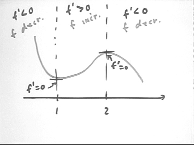
Sketch the graph of a continuous function f(x) with the following properties:
As indicated in the figure below f ' > 0 on (1, 2) means that f must be increasing on (1, 2); f ' < 0 on (0, 1) and (2, 3) means that f is decreasing on those intervals. f ' (x) = 0 at x = 1 and x = 2 means that the graph of f must 'level off' at those points.
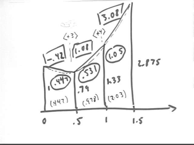
Sketch and completely label a Trapezoidal Approximation Graph for f(x) = x^3/3 + x^2 - x + 1 on the interval 0 < x < 1, using interval length .5. Be sure to include rate of slope change.
We easily evaluate the function, obtaining approximate values 1, .79, 1.33, 2.88 at x = 0, 1, 1.5. Note that in this solution we extend the graph to x = 1.5; your work need only have extended up through x = 1, with only the first two of the three trapezoids we will obtain here.
The slopes -.42, 1.08 and 3.08 are easily calculated, as are the areas .448, .531 and 1.052. Adding the areas thru the end of each trapezoid we get the accumulated areas .448, .979 and 2.03.
Dividing the slope change by the interval `dx = .5 at at x = .5 and at x = 1 yields rates of slope change +3 and +4.
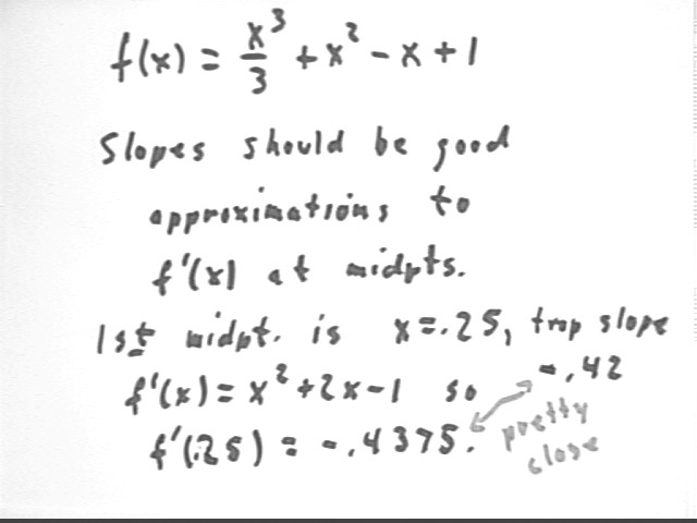
The slopes of the graph represent average slope corresponding to each of the three intervals. We can compare the average slopes to the midpoint slopes. The midpoint slopes would be obtained by taking the derivative at each midpoint.
The derivative function is easily found to be f ' (x) = x^2 + 2 x - 1. The midpt value on the first interval will be f ' ( .25 ) = -.4375, which is close to the trapezoidal approximation -.42. The other midpoint values are shown in context of the DERIVE commands.
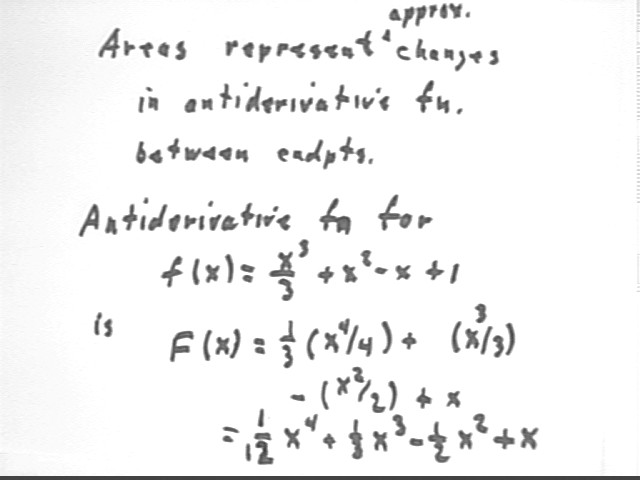
We let F(x) represent an antiderivative function for f(x). The area of a trapezoid represents the approximate change in the antiderivative function F(x) between the two endpoints of the trapezoid.
Reversing the derivative process we find an antiderivative function F(x) = 1/12 x^4 + 1/3 x^3 - 1/2 x^2 + x. You should check to be sure that the derivative of F(x) = 1/12 x^4 + 1/3 x^3 - 1/2 x^2 + x is indeed F'(x) = f(x) = x^3 / 3 + x^2 - x + 1.
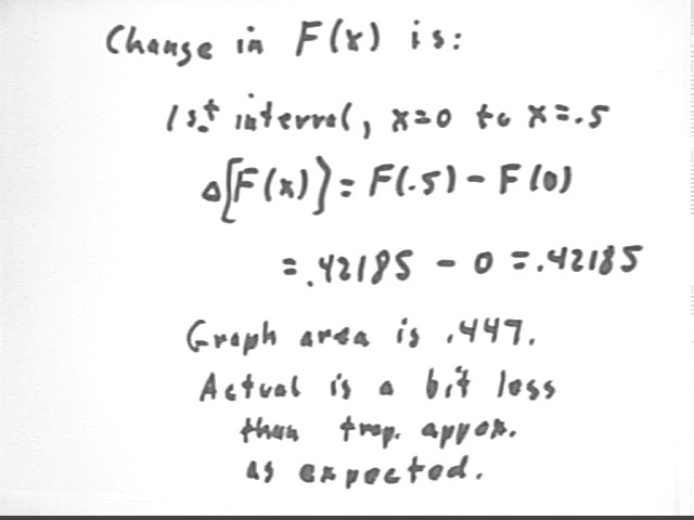
The change in the antiderivative function F(x) from x = a to x = b is just the change in the values of F(x) from x = a to x = b, i.e., final value - initial value = F(b) - F(a).
For the first interval, from x = 0 to x = .5, we see that F(x) changes from F(0) = 0 to F(.5) = .42185, a change of .42185. This compares with the area .448 of the trapezoidal approximation graph.
Since the curve of the actual function is concave up we expect that the actual area will be less than the trapezoidal approximation, as was the case here.
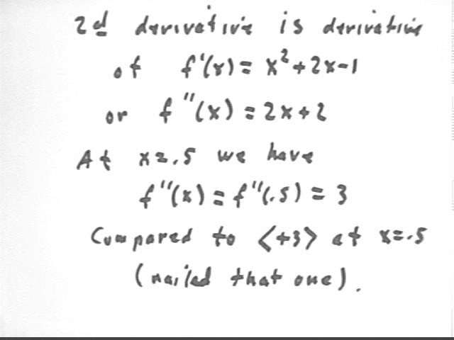
The rate of slope change is the average rate at which the (average) slope changes. The slope approximates the derivative and the average rate at which the slope changes approximates the rate of change of the derivative, which would be the second derivative.
The second derivative of our f(x) function is easily calculated and evaluated at x = .5, We obtain f '' (.5) = +3. This is in perfect agreement with the trapezoidal approximation to the rate of slope change for x = .5. The perfect agreement is a result of the linearity of the rate of slope change function f '' ( x) = 2x + 2.
Compare this with the fact that the average slopes of a quadratic function will be exactly equal to midpoint slopes, due to the linearity of the derivative of the quadratic function. In this case the rate of slope change function, the second derivative, is linear resulting in a perfect approximation to the rate of slope change. Note that this happens when and only when the original function is a cubic polynomial (the only function whose second derivative is linear is a cubic polynomial).
Our function f(x) is increasing from x = .5 thru x = 1.5. The following development depends on the fact that our function be either increasing or decreasing throughout the interval being considered. These results will be extended later to functions which are not monotone (i.e., strictly increasing or strictly decreasing).
Note the DERIVE commands for evaluating these quantities:
VECTOR(x^3/3 + x^2 - x + 1, x, 0, 1.5, 0.5) instructs the program to evaluate x^3/3 + x^2 - x + 1 at x values from 0 to 1.5 by step 0.5 and yields the following:
[1, 0.7916666666, 1.333333333, 2.875]. These are the function values at x = 0, .5, 1, 1.5, 2.
f(x) := x^3/3 + x^2 - x + 1 defines the function f(x).
VECTOR((f(x + .5) - f(x ))/0.5, x, 0, 1, .5) evaluates the expression (f(x+.5) - f(x) ) / .5 for x values from 0 to 1 by step .5. The x values will thus be 0, .5 and 1.
For x = 0 we see that (f(x+.5) - f(x) ) / .5 gives us (f(0+.5) - f(0) ) / .5 = (f(.5) - f(0) ) / .5, which we see as the rise / run for the first trapezoid, and also as the difference quotient {f(x+`dx) - f(x)) / `dx for x = 0 and `dx = .5.
We interpret the expression similarly for x = .5 and x = 1, seeing that the expression gives us the slopes of the second and third trapezoids.
The command yields the following:
[-.42, 1.08, 3.08 ]. These are the slopes of the three trapezoids.
VECTOR((f(x) + f(x - 0.5))/2�0.5, x, 0.5, 1.5, 0.5) evaluates the expression (f(x+.5) + f(x) ) * .5 for x values from 0 to 1 by step .5. The x values will thus be 0, .5 and 1.
For x = 0 we see that (f(x+.5) + f(x) ) * .5 gives us (f(0+.5) + f(0) ) * .5 = (f(.5) + f(0) ) * .5, which we see as the ave graph altitude * trapezoid width for the first trapezoid, giving us the area of the first trapezoid.
We interpret the expression similarly for x = .5 and x = 1, seeing that the expression gives us the areas of the second and third trapezoids.
The command yields the following:
[0.4479166666, 0.53125, 1.052083333]. These are the areas of the three trapezoids.
fDer(x) := x^2 + 2�x - 1 defines the function fDer(x) to be x^2 + 2x - 1, which is the derivative of the f(x) function.
VECTOR(fDer(x), x, 0.25, 1.25, 0.5) evaluates the derivative function at x values from .25 thru 1.25 by interval `dx = .5, yielding
[-0.4375, 1.0625, 3.0625]. These are the values of the derivative of the actual function at the midpoints of the three intervals.
(INT(f(x), x, a, a + 0.5) stands for the integral of f(x) from x = a to x = a + .5. The integral of a function between two given points is evaluated by finding an antiderivative (the 'change-in-amount' function for a rate function f(x) in the flow model) and determining the change in the antiderivative (i.e., the change in the amount) between the two x values.
VECTOR(INT(f(x), x, a, a + 0.5), a, 0, 1,.5) evaluates (INT(f(x), x, a, a + 0.5) for a values from 0 to 1.5 by interval `dx = .5.
For a = 0 this command evaluates (INT(f(x), x, 0, 0 + 0.5) = INT(f(x), x, 0, 0.5). This will be the actual area under the f(x) curve from x = 0 to x = .5.
For a = .5 this command evaluates (INT(f(x), x, .5, .5 + 0.5) = INT(f(x), x, .5, 1). This will be the actual area under the f(x) curve from x = .5 to x = 1.
For a = 1 this command evaluates (INT(f(x), x, 1, 1 + 0.5) = INT(f(x), x, 1, 1.5). This will be the actual area under the f(x) curve from x = 1 to x = 1.5.
The command yields
[0.421875, 0.4947916666, 1.005208333]. These values represent the actual areas under the f(x) curve for the intervals corresponding to the 3 trapezoids.
[0.421875, 0.4947916666, 1.005208333]. These values represent the actual areas under the f(x) curve for the intervals corresponding to the 3 trapezoids.
Instead of doing a trapezoidal approximation to the areas under our graph we do rectangular approximations. We first do a 'lower' rectangular approximation by using the left-hand value of f(x) on each interval, obtaining the red-shaded regions with areas .395 and .665, giving approximation 1.06 to the total area.
This approximation corresponds, for example, to application of the initial velocity as opposed to the approximate average velocity (as in the trapezoidal approximation) to the entire interval, or using the initial flow rate rather than the average flow rate over an interval.
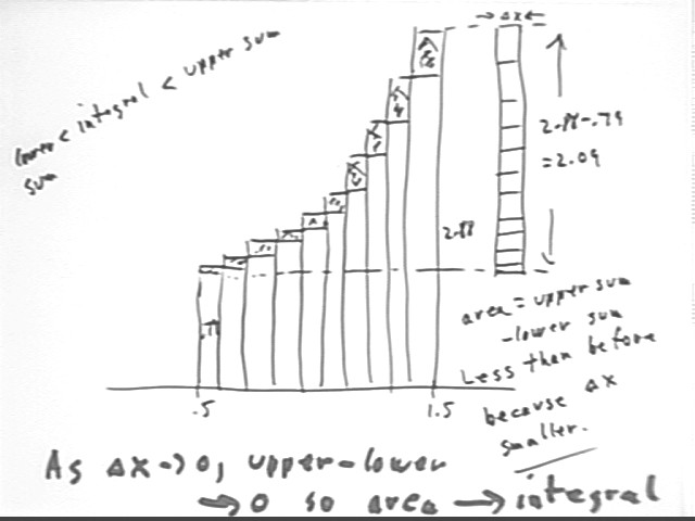
We then do an 'upper' rectangular approximation (corresponding here to using, for example, only the final velocity rather than an average velocity), obtaining areas .665 and 1.44 and giving approximate total area 2.11.
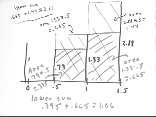
We observe that the trapezoidal area is less than the upper estimate and greater than the lower estimate. We observe also that if the function is increasing, which prevents it from 'dipping below' the lower-estimate value or exceeding the upper-estimate value, its integral between x=.5 and x=1.5 will also be confined between the two estimates.
The difference between the lower and upper estimates is the total area of the shaded rectangles. These rectangles are reconstructed to the right of the graph, in such a way as to show that their total area depends only on f(.5) = .79 and f(1.5) = 2.88, and on the width `dx = .5 of the interval of the approximation.
Note that the total area of the shaded rectangles is [f(b) - f(a) ] * `dx = [ f(1.5) - f(.5) ] * .5 = [ 2.88 - .79 ] * .5 = 1.05 approx.. This tells us that the upper and lower sums differ by 1.05.
It follows that the actual integral can differ from either upper or lower sum by no more than 1.05.
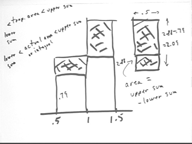
Had we broken the approximation into smaller intervals the small 'error rectangles' depicted below.
We note that the total area of these rectangles, which are collected to the right of the graph into a single rectangle whose width is `dx and whose altitude is still [ f(b) - f(a) ] = [ f(1.5) - f(.5) ] = (2.88 - .79) = 2.09, is less than before. In this case the total area of the 'error rectangles' is [ f(b) - f(a) ] * `dx = 2.09 * `dx.
It follows that the integral can differ from the upper sum or from the lower sum by at most 2.09 * `dx.
Since we can make `dx as small as we wish, we conclude that the either the upper sum or the lower sum can be made as close to the actual integral as we wish.
So the limit as `dx -> 0 of the lower sum is equal to the integral.
And the limit as `dx -> 0 of the upper sum is equal to the integral.