Calculus I Quiz 1021
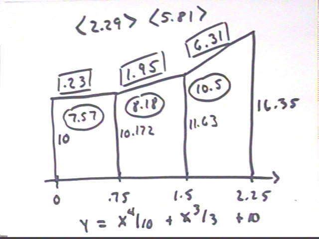
Sketch a trapezoidal approximation graph for y = x^4 / 10 + x^3 / 3 + 10 for 0 <= x <= 2.25, using increment `dx = .75.
The graph is shown here without comment. Review previous notes if it isn't clear how the graph is constructed and labeled.
Demonstrate how well the slopes represent midpoint derivative, how well the areas represent the appropriate integrals, and how well the rates of slope change represent the second derivatives. Discuss why the approximations should be slightly different from the actual values and why they are greater or less than the actual values, as the case may be.
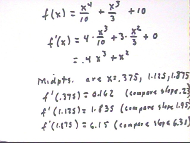
Evaluating the derivative f ' (x) = .4 x^3 + x^2 at the midpoints x = .375, 1.125 and 1.875 of the trapezoids we find that the derivatives are less closely approximated with each succeeding trapezoid (the respective discrepancies are .07, .12 and .16). This is due to the increasing rate of change of the slopes, which imply greater slope change on the right-hand half of the trapezoid than the left so that the midpoint slope is less than the average slope.
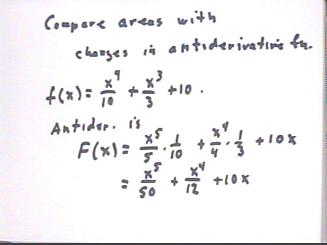
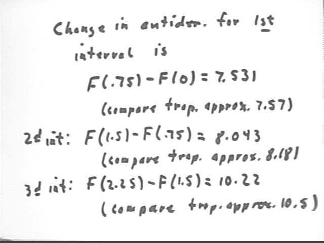
Recallling how the change-in-amount function is an antiderivative of the rate function, and how the change in amount is represents by the area under the rate curve, we understand that the areas should be equal to the changes in an antiderivative function. Using antiderivative F(x) = x^5 / 50 + x^4 / 12 + 10 x we get changes of 7.531, 8.043 and 10.22 for the three trapezoids.
These numbers represent the actual areas under the f(x) curve, which are closely approximated by the trapezoidal areas. The approximation is closer for the first trapezoid (difference of .04 approx.) than for the second (difference about .14) and still less close for the third (difference about .28). This is again due to the increasing rate of increase of the slopes, which means that the actual curve always lies below the trapezoid and more so for greater rate of slope increase.
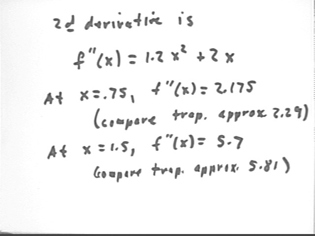
The second derivative function is f '' ( x) = 1.2 x^2 + 2 x, which as we see is well approximated at x = .75 and at x = 1.5 by the rates of slope change.
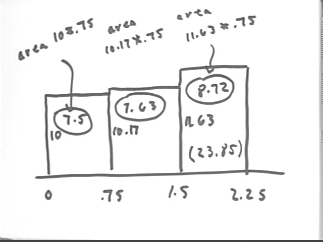
Do a lower and an upper Riemann sum and determine the difference between the two.
Our Riemann sums use upper or lower rectangles instead of trapezoids. The approximation of either Riemann sum is not as good as that of a trapezoidal graph, but we can use Riemann sums to prove that the integral of a continuous function must indeed approach a limit. This proof would be more difficult with trapezoids.
Since the graph is increasing we obtain the lower sum by using the left-hand endpoints as indicated below. The final accumulated area 23.85 of the rectangles is indicated with the usual labeling conventions.
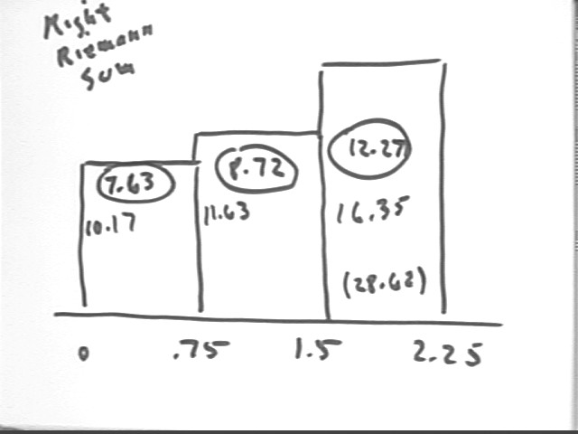
Since the graph is increasing we obtain the upper sum by using the right-hand endpoints as indicated below. The final accumulated area 28.62 of the rectangles is indicated with the usual labeling conventions.
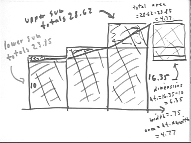
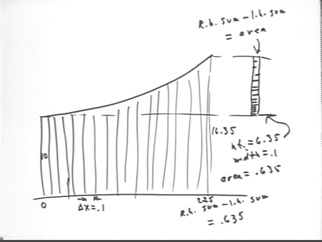
We see in the graph below how the discrepancies between upper and lower sum are represented by the areas of 3 small rectangles, on at the 'top' of each individual rectangle. If these rectangles are 'stacked' as shown to the right we see why their total area is equal to this discrepancy. The total area is just the change in function value from its left-hand extreme value of 10 to its right-hand maximum of 16.35, multiplied by the width of a single interval.
What would the difference be if we had used an increment of .1?
As shown below the total area will again be just the change in function value from its left-hand extreme value of 10 to its right-hand maximum of 16.35, multiplied by the width of a single interval. The difference is that in this case the single interval has width .1, so the discrepancy is only 6.35 * .1 = .635, as opposed to 4.77 with the preceding interval of .75.
You might note that .1 really isn't a good interval width to use if we're trying to subdivide the larger interval 0 < x < 2.25. However the principle of the explanation should be clear.
Riemann Sum notation:
The general Riemann sum is expressed here in terms of an unspecified function f(t), unspecified t coordinates a and b and an unspecified number n of equal subintervals.
The length of the entire interval is b - a, and each of the n subintervals has length `dt = (b - a) / n.
The points run from t0 = 1 to tn = b, and are labeled t0, t1, t2, ..., tn.
We would calculate the left-hand sum by using the left-hand 'graph altitude' corresponding to each interval (corresponding, for example, to using the initial velocity on each interval to calculate the corresponding displacement).
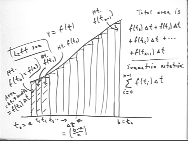
The total area is thus f(t0) * `dt + f(t1) * `dt + f(t2) * `dt + ... + f(t(n-1)) * `dt.
This is expressed in summation notation as indicated in the above figure. In typewriter notation the summation is expressed as SUM( f(ti) * `dt, i, 0, n-1) ), meaning that for an index i which runs from 0 to n-1 we calculate f(ti) * `dt; we then sum up all these results. That is,
When we sum these results we get our previous result f(t0) * `dt + f(t1) * `dt + f(t2) * `dt + ... + f(t(n-1)) * `dt.
| x | f(x) | slope | area | rate of slope change |
| 0 | 10 | |||
| 0.75 | 10.172266 | 0.23 | 7.565 | 2.2875 |
| 1.5 | 11.63125 | 1.945 | 8.176 | 5.8125 |
| 2.25 | 16.359766 | 6.305 | 10.5 | |
| midpt | midpoint derivative | actual area under fn | second derivative | |
| 0.38 | 0.162 | 7.531 | 2.175 | |
| 1.13 | 1.835 | 8.043 | 5.7 | |
| 1.88 | 6.152 | 10.22 | ||
| left Riemann area | right Riemann area | difference right - left | ||
| 7.5 | 7.629 | 0.129 | ||
| 7.6291992 | 8.723 | 1.094 | ||
| 8.7234375 | 12.27 | 3.546 | ||
| Sums | 23.852637 | 28.62 | 4.77 | |
| right - left | 4.77 | |||
Text Section 5.2
Section 5.2 Problems 2, 4, 7, 10, 13, 16, 21, 23, 24, 28, 29, 32, 37
Text Section 5.3
Section 5.3 Problems 2, 4-7, 10, 12, 16, 19, 20, 22, 25, 26
Text Section 5.4
Section 5.4 Problems 2, 4, 5, 8-21