Calculus I Quiz 1023
Construct a trapezoidal approximation graph for y = f(x) = 1 + (x-1)^4 for 0 < x < .9, using increment .3. Note that the expanded form of this function is y = f(x) = x^4 - 4x^3 + 6 x^2 - 4 x + 2; you will probably find the function easier to evaluate in the first form.
What is the approximation of your graph to the integral of this function from x = .3 to x = .9?
Area from .3 to .9 = area from 0 to .9 - area from 0 to .3
= accum area thru 3d trap - accum area thru 1st trap = ... = .684.
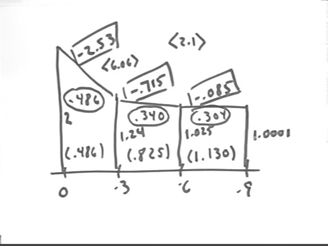
| x | y | slope | area | accum area | slope change rate | midpt | y' at midpt | integral on interval | integral to pt | y'' |
| 0 | 2 | |||||||||
| 0.3 | 1.2401 | -2.533 | 0.486015 | 0.486015 | 6.06 | 0.15 | -2.4565 | 0.466386 | 0.466386 | 5.88 |
| 0.6 | 1.0256 | -0.715 | 0.339855 | 0.82587 | 2.1 | 0.45 | -0.6655 | 0.331566 | 0.797952 | 1.92 |
| 0.9 | 1.0001 | -0.085 | 0.303855 | 1.129725 | 0.3 | 0.75 | -0.0625 | 0.302046 | 1.099998 | 0.12 |
Using the usual methods we obtain the graph depicted below.
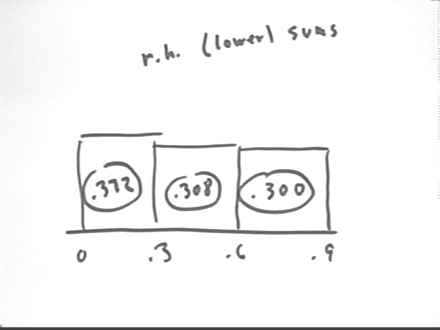
What are the lower and upper Riemann sums approximating the integral of this function from x = .3 to x = .9, using `dx = .3?
Using the right-hand approximation on each interval we arrive at the right-hand Riemann sum. Since the function is decreasing the right-hand sum will be the lower sum. For the entire graph we obtain a total of .372 + .308 + .300 = .980.
For the interval from .3 to .9 we obtain lower sum .308 + .300 = .608.
The left-hand sum will be the upper sum, which for the whole graph totals 1.28.
For the interval from .3 to .9 the upper sum is .372 + .308 = .680.
Note that for the interval from .3 to .9 the difference between the sums is .680 - .608 = .72, which at it must be is equal to
| f (.9) - f(.3) | * .3 = | 1.0001 - 1.24 | * .3 = .072.

The table below indicates these results:
| x | y | upper rect | lower rect |
| 0 | 2 | 0.6 | 0.37203 |
| 0.3 | 1.2401 | 0.37203 | 0.30768 |
| 0.6 | 1.0256 | 0.30768 | 0.30003 |
| 0.9 | 1.0001 | ||
| totals: | 1.27971 | 0.97974 |
What is the actual value of the integral of this function from x = .3 to x = .9?
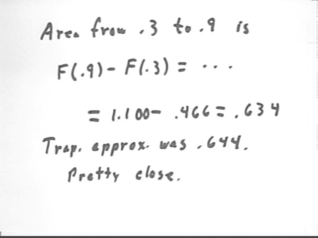
We approximate the integral by as the of the trapezoidal approximation from x = .3 to x = .9, which we see is the change in accumulated area from x = .3 thru x = .9. The approximation of our trapezoidal graph is therefore 1.130 - .486 = .644.
This is of course equal to the sum of the trapezoidal areas from .3 to .6, and from .6 to .9.
From this we understand that the integral from .3 to .9 is the sum of the integrals from .3 to .6 and from .6 to .9.
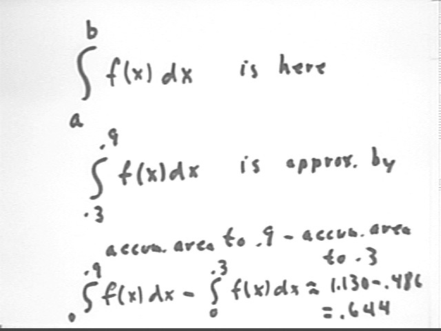
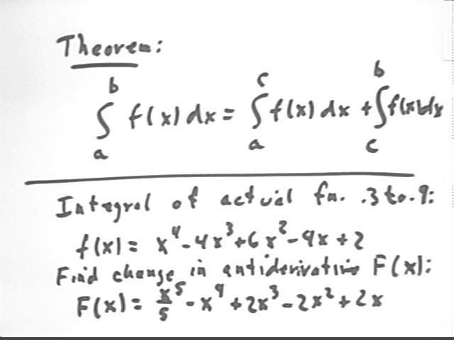
This illustrates an important general property of integrals, that the integral from a to b is equal to the sum of two integrals, one from a to c and the other from c to b.
Now we turn to finding the integral of the actual function from .3 to .9.
We evaluate the integral by finding the change in the change-in-amount function, or the antiderivative function, between x = .3 and x = .9.
The antiderivative of f(x) = x^4 - 4x^3 + 6 x^2 - 4 x + 2 is F(x) = x^5/5 - x^4 + 3 x^3 - 2 x^2 + 2 x.
Thus the area is F(.9) - F(.3), which we easily evaluate to obtain .634, accurate to 3 significant figures.
How much discrepancy is there between the lower Riemann sum and the actual integral? Answer the same question for the upper Riemann sum.
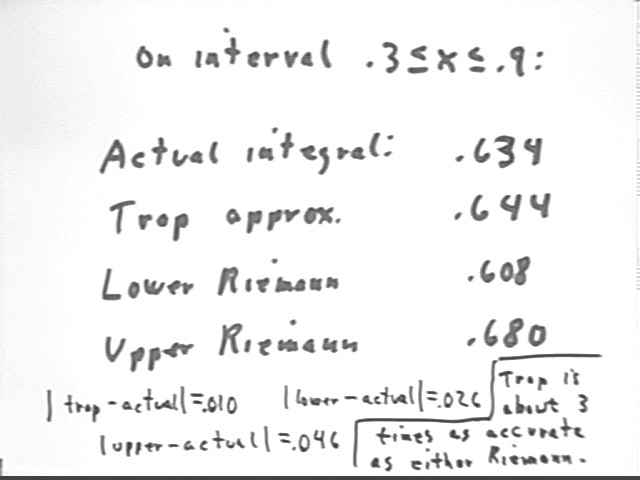
Summarizing our results so far we can compare the actual integral with the trapezoidal approximation, as well as with the lower and upper Riemann approximations.
The magnitude of the difference between the trapezoidal approximation and the actual integral is easily seen to be .010.
The magnitude of the difference between the trapezoidal approximation and the actual integral is seen to be .026.
The magnitude of the difference between the trapezoidal approximation and the actual integral is seen to be .046.
The closer of the two Riemann sums is nearly 3 times as far from the actual value as the trapezoidal approximation.
Which Riemann sum is closer to the actual integral and why?
The lower sum is closer to the actual value, lying within .026 compared to the discrepancy of .046 between the upper sum and the actual value.
This results from the upward concavity of the graph (i.e., the increasing derivative, the positive second derivative).
How many times closer is the trapezoidal approximation to the integral than the closer of the two Riemann sums?
As seen above the trapezoidal approximation is 2.6 times, or about 3 times, bettern than the closer of the two Riemann sums.
What interval would be necessary before the closer of the two Riemann sums would be as close to the actual integral as the trapezoidal approximation?
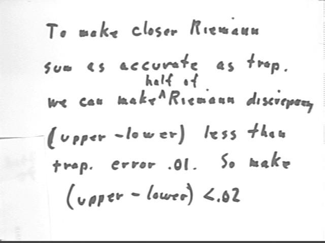
If the upper and lower Riemann sums differ by a certain amount, then because the actual integral lies between these sums the closer of the two Riemann sums will differ from the actual integral by no more than half this amount.
So to guarantee that the closer of the two Riemann sums be within the trapezoidal 'error' of .01, it suffices to make the difference between the upper and lower Riemann sums less than .02.
We recall that for an increasing or a decreasing function the difference between upper and lower Riemann sums is represented by the area of a rectangle whose width is equal to the subinterval length `dx and whose height is equal to the difference between the initial and final function values. For this specific function on the given interval the initial and final function values differ by about .24 so we have
upper - lower = .24 * `dx.
We want upper - lower to be < .2 so we solve
.2 < .24 * `dx for `dx to get
`dx = .2 / .24 = .0833... .
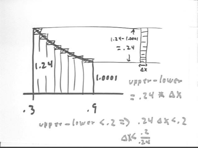
It follows that for `dx < .0833... the upper and lower sums will differ by < .2, meaning that the closer of the two Riemann sums will lie within .1 of the actual integral.
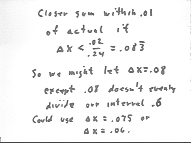
Note however that .0833... is not a good choice for `dx, since it won't partition the interval from .3 to .9 into a whole number of equal intervals (i.e., .9 - .3 = .6 is not evenly divisible by .0833... ).
So we have to choose something less than .0833... . .08 would be convenient but it doesn't evenly divide into .6.
.075 divides the interval evenly into 8 subintervals and would be a feasible choice.
.06 would be another reasonable choice.
Either of these intervals would result in a difference of < .2 between lower and upper sum and would therefore guarantee that the closer of the Riemann sums be within .1 of the actual integral.
The table below depicts all the information summarized in the trapezoidal graph and in the comparisons made throughout this analysis.
| x | y | slope | area | accum area | slope change rate | midpt | y' at midpt | integral on interval | integral to pt | y'' |
| 0 | 2 | |||||||||
| 0.3 | 1.2401 | -2.533 | 0.486015 | 0.486015 | 6.06 | 0.15 | -2.4565 | 0.466386 | 0.466386 | 5.88 |
| 0.6 | 1.0256 | -0.715 | 0.339855 | 0.82587 | 2.1 | 0.45 | -0.6655 | 0.331566 | 0.797952 | 1.92 |
| 0.9 | 1.0001 | -0.085 | 0.303855 | 1.129725 | 0.3 | 0.75 | -0.0625 | 0.302046 | 1.099998 | 0.12 |
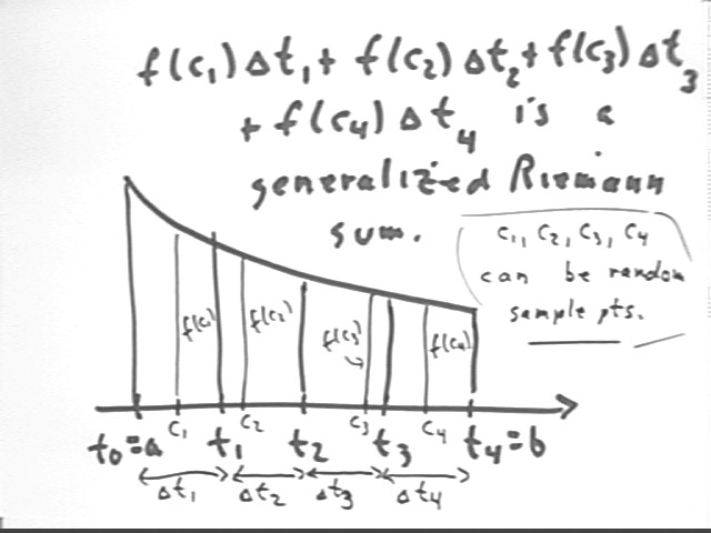
A generalized Riemann sum can use a 'sample point' c anywhere within each interval; evaluating the function at this point, and multiplying by the interval width, gives us a result that will lie between the lower and upper estimate for that interval.
In the figure below we have 4 intervals, partitioned by t0 = a, then by t1, t2, t3 and t4 = b. In the ith interval we have the sample point ci, giving us function value f(ci).
The intervals in a generalized Riemann sum need not be uniform. It is sometimes desirable in both application and theory to use intervals of different widths, or of unspecified widths. For this reason we use `dt1, `dt2, `dt3, etc.. for the intervals, and we write the Riemann sum as f(c1) `dt1 + f(c2) `dt2 + f(c3) `dt3 + f(c4) `dt4.
For an unspecified number n of subintervals we would write SUM ( f(ci) * `dti, i, 1, n), meaning the sum of terms f(ci) * `dti for index i running from 1 to n.
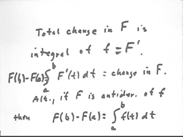
The text tells us that the total change in the value of a function F(t) between two values of t is equal to the integral of its derivative f (t) = F ' (t).
We have encountered this statement in terms of a rate function f(t) and its antiderivative function F ' (t). We know that the change in the antiderivative function is the change in the amount, represented by the area under the curve. Our statement has been that F(b) - F(a) = INT( f(t), t, a, b).
Since f(t) = F ' (t) the two statements are identical.
If f(t) represents a rate-of-depth-change function then the change in depth between t = a and t = b will be equal to the integral of f(t) between t = a and t = b, represented by the area under the rate f(t) vs. clock time t graph.
What therefore is the average rate of depth change, with respect to t, for rate function f(t) between t = a and t = b?
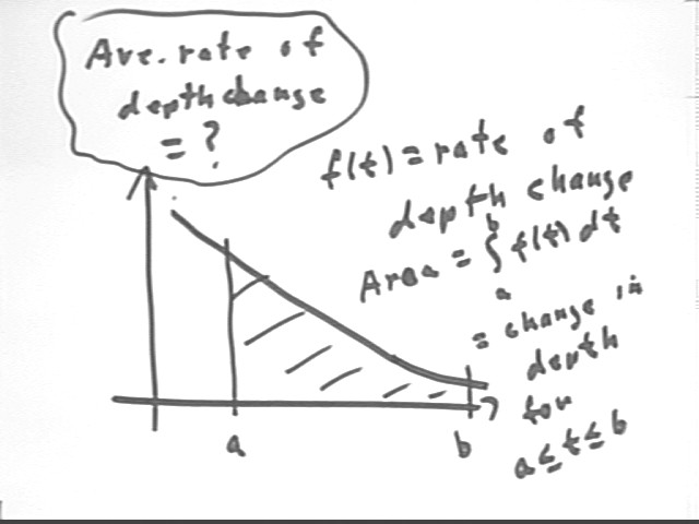
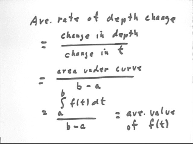
Ave. rate of change of depth with respect to t is
ave rate = change in depth / change in t.
Change in depth is represented by the area under the curve, which is the same as the integral of the function f(t) with respect to t, from t = a to t = b.
The average rate is the average value of the rate function f(t), so we see that
ave value of f(t) = integral of f(t) for the given t interval, divided by the t interval (in this case `dt = b - a).
It follows that the integral is the product of the average value of f(t) and `dt= b-a.
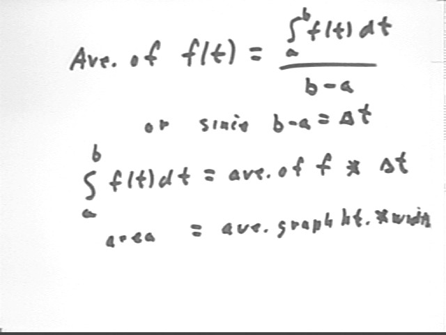
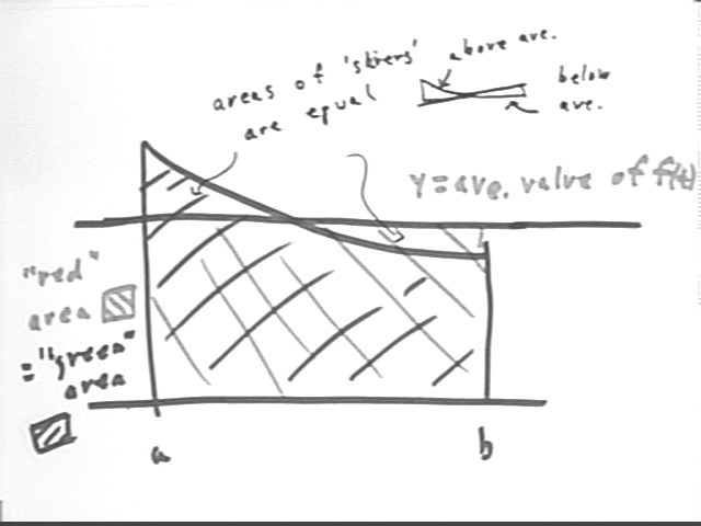
This is represented by the graph shown in the figure below. The horizontal line represents the average value of f(t). The area of the 'red' or 'backward-shaded' rectangle which lies between the t axis and this line represents ave value of f(t) * t interval = fAve * (b - a).
Since fAve * (b - a) is equal to the integral of the f(t) function, this rectangle has the same area and the 'green' or 'forward-shaded' region under the curve.
The small figure at upper right represents the fact that the 'sliver' under the f(t) graph and above the average value must be equal in area to the 'sliver' beneath the average value and above the f(t) graph. This is the condition necessary for the area of the region under the f(t) graph to be equal to the area of the 'ave-value' rectangle.