Calculus I Quiz 1118
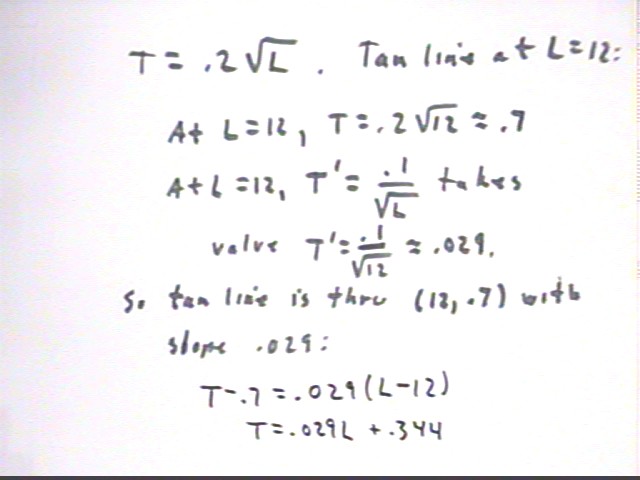
The period of a pendulum is T = .2 sqrt(L).
We calculate the equation of the tangent line by first finding the coordinates of the point and the slope of the tangent line, after which we will easily find the equation of the line.
Evaluating T and L = 12 we obtain t = .7, approx.
Using the power function rule we obtain T ' = .1 / sqrt(L), which when L = 12 gives us T ' = .029, approx..
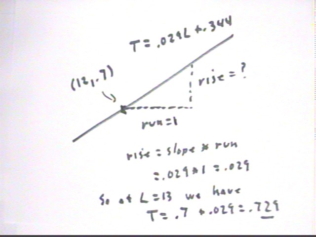
We then easily obtain the approximate equation of the tangent line: T = .029 L + .344.
The graph below depicts the tangent line and the curve representing T = .2 sqrt(L). You should know what the square-root graph looks like.
The second figure below shows the accurate graph.
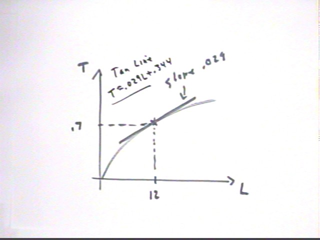
The figure below represents the tangent line in the vicinity of the point (L , T) = (12, .7).
We wish to find the approximate change in T due to a change from L = 12 to L = 13. If we use the tangent line to calculate this change, we will have to move 'over' `dL = 1 unit from the L = 12 point.
The question is now how much change in T will correspond to this unit chnage in L. Since the slope of the tangent line is .029 we easily determine that T will change by `dT = slope * run = .029.
So we predict that at L = 13 we will have T = .729.
Timing 10 cycles of a 12 cm pendulum then repreating for a 13 cm pendulum we find that this result appears to be very plausible.
We also predicted the change in L necessary to change T by .1 second. We see that `dT / `dL = .029 so that `dL = `dT / .029, so to change T by `dT = .1 we need `dL = .1 / .029 = .34, approx.. Adding .34 cm to the 12 cm length we get a 15.4 cm pendulum, whose period when measured appeared indistinguishable from the .8 sec.
At point (L, T) the slope will be T ' = .1 / sqrt(L), so we have a line thru (L, .2 sqrt(L) ) with slope .1 / sqrt(L).
The slope of this line is .1 / sqrt(L), so `dT / `dL = .1 / sqrt(L), approx. If L changes by `dL we will have `dT = slope * `dL = .1 / sqrt(L) * `dL = .1 `dL / sqrt(L).
The next question concerns the question of which of two functions approaches zero faster:
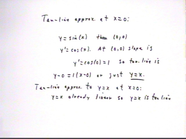
We easily find the tangent-line approximations to be y = x and y = x.
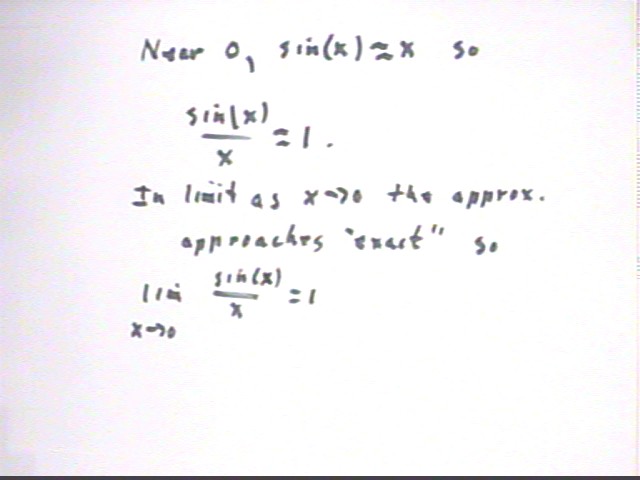
Thus close to x = 0 we see that sin(x) / x is close to x / x. In the limit at x ->0 this ratio approaches x / x = 1.
The figure below depicts the y = sin(x) and y = x curves, showing how the two 'join' as x -> 0.
The next question again concerns the question of which of two functions approaches zero faster:
We should first graph the two functions. It is very important to be able to construct such graphs.
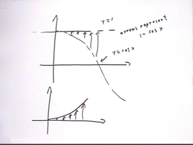
We construct the graph of y = 1 - cos x by first sketching the y = 1 and y = cos(x) graphs. Then 1 - cos(x) is represented for any x by an arrow extending from the graph of y = cos x to the graph of y = 1, as depicted in the first graph.
The second graph depicts the function defined by those 'arrows' which represent the differences. This will be the graph of y = 1 - cos(x).
We construct the graph of y = 1 - e^x by first sketching the y = 1 and y = e^x graphs. Then 1 - e^x is represented for any x by an arrow extending from the graph of y = e^x to the graph of y = 1, as depicted in the first graph. Note that since e^x > 1 the differences are negative, as the downward pointing arrows indicate.
The second graph depicts the function defined by those 'arrows' which represent the differences. This will be the graph of y = 1 - e^x.
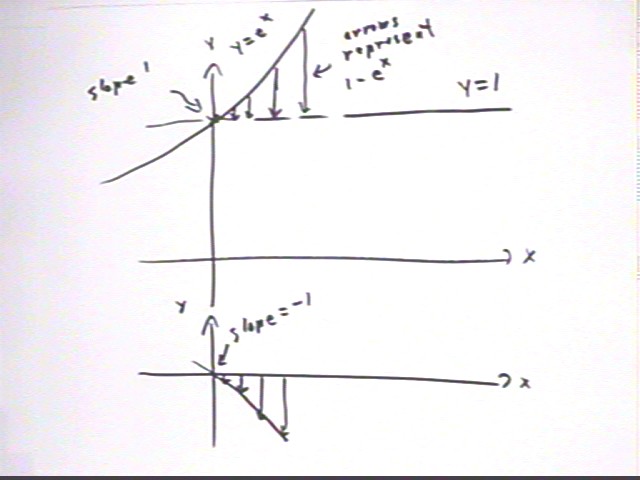
Now we find the equations of the tangent lines. These equations are easily see to be y = 0, for the y = 1 - cos(x) function, and y = -x for the y = e^-x function.
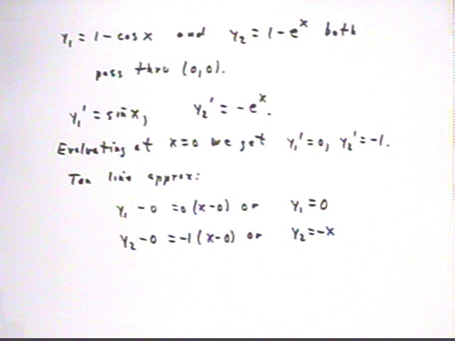
The graph below depicts the functions with their tangent lines. The tangent line y = 0 for the first function coincides with the x axis.
We can try to estimate from the graph what happens at various values of x. The figure below depicts the graphs of the two function with their tangent lines (note that the tangent line for the first function coincides with the x axis).
At any given x value the values of the two functions can be represented by arrows from the x axis to the graphs. We see that for a certain x value the first function appears to be about 1/6 as far from the x axis as the second, and since one function is negative while the other is positive we conclude that for this x the ratio (1 - cos(x) ) / (x - e^x) is about -1/6.
Moving closer to x = 0 we see that both functions get closer to 0, but it's not entirely clear what happens to the ratio.
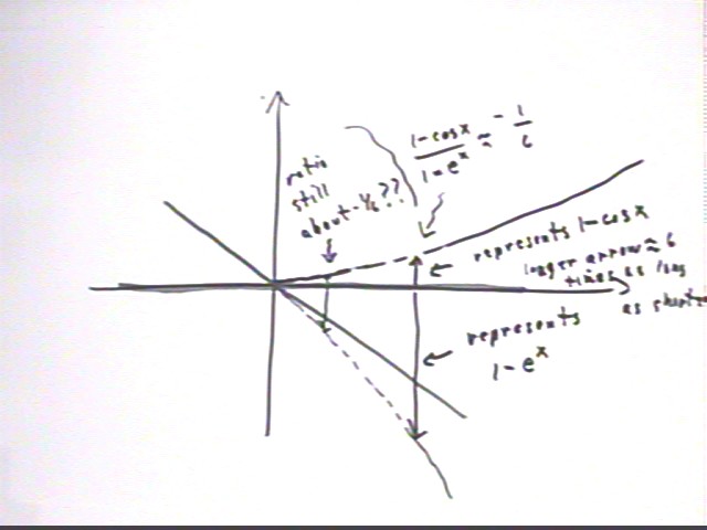
The hand sketch above isn't as accurate as the graph shown below. However it still might not be entirely clear what happens to the ratio of the two values as x -> 0.
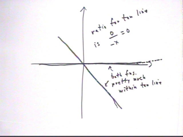
The figure below shows what happens if we 'zoom in' nearer to x = 0. We see that the first function stays very close to its tangent line at the x axis while the second stays very close to its tangent line y = -x.
This figure shows that the value of the first function is effectively zero for small x (i.e., very nearly equal to the tangent-line value y = 0), while the value of the second is very nearly equal to the value of the tangent-line function y = -x.
The ratio of values for the tangent lines y = -x and y = 0 is 0 / (-x) = 0. Since as x -> 0 each function approaches its tangent-line value it follows that the ratio of the functions approaches the ratio of the tangent-line values, so the limiting ratio is zero.
That is, the limit as x -> 0 of (1 - cos(x) ) / (1 - e^x) is 0.
This behavior occurs generally. Whenever two function both approach zero and the same x value, the limiting value of the ratio is equal to the limiting value of the tangent-line approximations, provided the derivatives of both function are defined at that point (gotta have the derivative to make the tangent line). So the limiting ratio of the two functions is equal to the limiting ratio of their derivatives.
Comparing y = 1.001^x with y = x^1000, which function 'wins' as x -> infinity?
Infinite limits obey the rule analogous to the rule for finite limits, as you text will indicate.
The graph of y = x^1000 'takes off' very rapidly, while the graph of y = 1.001^x grows very slowly, for any familiar range of x values. Comparing the x = 100 values of these functions we see that the first will be y = 100^1000, which will consist of 1 followed by 2,000 zeros, while the second will be y = 1.001^100 = 1.105, approx. It certainly appears that the first function should continue to 'beat' the second by an astounding margin.
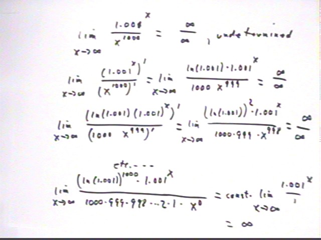
However if we try to take the limit as x -> infinity of the ratio 1.001^x / (x^1000) we find that both the exponential and the power function do indeed approach infinity, despite the fact that the power function appears to approach infinity much more quickly.
In the second line we see that the ratio of the derivatives also gives us the form inifinity/infinity. We note that the 'power' of the denominator is reduced when we take this ratio, while the numerator maintains its 1.001^x term.
In the third line we see that this process continues. By this time we see a pattern and conclude that the numerator will continue to contain the factor 1.001^x no matter how many derivatives we take, though it will also accumulate higher and higher powers of the small constant number ln(1.001). The power of the denominator will continue to decrease, the the denominator will collect as factors all the powers through which we have decreased.
By the time we get to power 0 in the denominator we will have the expression shown in the last line. ln(1.001)^1000 is a very small number and 1000 * 999 * 998 * ... 2 * 1 is a very large number so we have the final ratio ln(1.001)^1000 / ( 1000 * 999 * 998 * ... 2 * 1 ) * 1.001^x. The constant term ln(1.001)^1000 / ( 1000 * 999 * 998 * ... 2 * 1 ) is an astoundingly small number, but it's fixed and won't change as x increases. So we can make 1.001^x as large as we wish by choosing x to be large enough and we can therefore make ln(1.001)^1000 / ( 1000 * 999 * 998 * ... 2 * 1 ) * 1.001^x as large as we wish.
It follows that the limiting value of this expression as x -> infinity is therefore infinite.
This tells us that the original limit as x -> infinity of 1.001^x / x^1000 is also infinite, meaning that if x is chosen large enough 1.001^x / x^1000 can be made as large as we desire.
Our conclusion is that 1.001^x eventually 'beats' x^1000 as badly as we might wish.
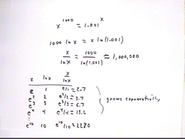
To further examine how it can be that 1.001^x eventually 'beats' x^1000 note that the two will be equal when x^1000 = 1.001^x, which as we see below happens when x / ln(x) is about 1,000,000. This doesn't tell us what x is but we can use a little informed trial and error to make an estimate.
If we let x values be powers of e we can easily calculate ln(x) values. As indicated in the table below for n = 1 to 10 we get values of x = e^n which when divided by the ln(x) values n give us ratios which at first increase slowly, then more and more quickly, until for x = e^10 the ratio is already in the thousands. This doesn't get us to the desired ratio around 1,000,000 but it shows that we can probably get there with little difficulty.
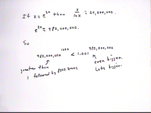
Using x = e^20 we obtain x / ln(x) = 24,000,000, well over the 1,000,000 we desire. So we expect that 1.001^x / x^1000 will be a lot more than the ratio 1 we were looking for.
x = e^20 = 480,000,000, approx.. Comparing the values of x^1000 and 1.001^x for x = 480,000,000 we see that while 480,000,000^1000 is a huge number (more than 1 followed by 8000 zeros, which is what we would get for 100,000,000^1000 = (10^8)^1000 = 10^8000) the number 1.001^480,000,000 is even bigger; in fact it's a lot bigger.