Calculus I Quiz 1202
It costs you $1000 to just operate your factory, plus $10 * sqrt(x) to produce x items.
If you produce x items then the price people are willing to pay for each is $10 * (1 - x/500).
If you produce 10 items how much money do you gain or lose?
Producing 10 items costs you $1000 + $10 * sqrt(10) = $1031, approx..
You sell those 10 items at $10 ( 1 - 10/500) = $9.80; total selling price is $98.
So your profit is $98 - $1031 =$933.
If you produce 300 items how much money do you gain or lose?
Producing 300 items costs you $1000 + $10 * sqrt(300) = $1173, approx..
You sell those 300 items at $10 ( 1 - 300/500) = $4; total selling price is 300 * $4 = $1200.
So your profit is $1200 - $1173 =$27.
What is the number of items that maximizes your profit or minimizes your loss?
If you produce x items then:
Machine tells us that this function maximizes around 242 items at $93.17.
You actually gotta know something to get the function to put into the machine.
However calculus is more efficient.
Our profit function is
P(x) = x ($10 (1-x/500) ) - $1000 - $10 sqrt(x)
= $ [ 10 x - 10 x^2 / 500 - 1000 - 10 sqrt(x) ].
The profit function maximizes where its derivative is zero.
P ' (x) = 10 - 10/500 * ( 2x ) - 0 - 10 * 1/(2 sqrt(x))
= 10 - .04 x - 5 / sqrt(x).
P ' (x) = 0 if
10 - .04 x - 5 / sqrt(x) = 0.
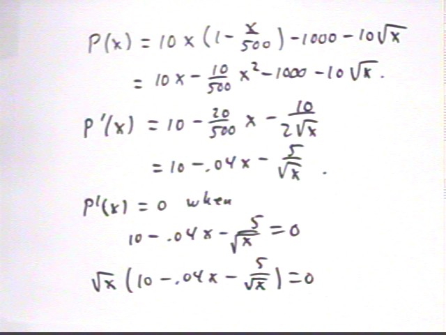
Multiplying both sides by sqrt(x) we get
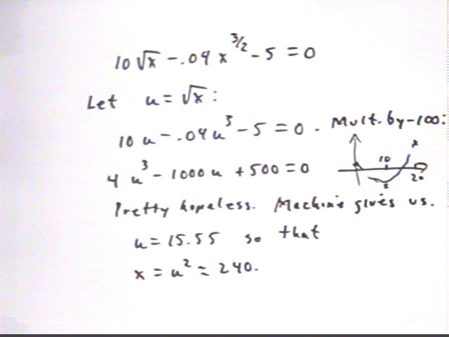
10 sqrt(x) - .04 x^(3/2) - 5 = 0 or
10 x^.5 - .04 x^1.5 - 5 = 0. Using u = sqrt(x) this is
10 u - .04 u^3 - 5 = 0; multiplying by -100 we have
4 u^3 - 1000 u + 500 = 0.
This expression is positive for u = 0, negative for u = 10 and positive for u = 20. We find that it is zero for u = -16, .5, 15.555.
u = sqrt(x) can't be negative so we ignore the u = -16.
Since x = u^2 we have zeros of P ' (x) at x = .5^2 and at x = 15.555^2.
x = 15.555^2 = 241.96, approx..
To see whether this is max or min look at P '' (x).
P''(x) = -.04 - 5 ( -1/2 * x^(-3/2) ) = -.04 + 2.5 x^(-3/2).
At x = 241.96 we have P '' (x) = -.04 + 2.5 / (241.96^(3/2) ). The term 2.5 / 241 would be about .01; 2.5 / (241)^(3/2) would be even less so we see that P '' (241.96) < 0.
Thus at x = 241.96 the graph is concave down, meaning that since P ' (x) is zero at this point the function must be a maximum at x = 241.96, approx..
The figure below depicts P ' (x) and P(x) both vs. x. We see that where P ' (x) is positive the graph of P(x) is increasing, where P ' (x) is negative the graph of P(x) is decreasing, and where P ' (x) is zero the graph of P(x) is 'level'.
Since the derivative P ' (x) goes from positive to negative as P ' (x) passed thru zero, the P(x) changes from increasing to decreasing at that point, ensuring that we reach a maximum at x = 241.96 approx.. This confirms the result of our second-derivative test.
The actual cost and revenue functions are shown in the figure below, with a restricted vertical scale. The cost function C = $1000 + $10 sqrt(x) is nearly linear for x > 150; the revenue function R(x) = x ( $10(1-x/500) ) = $10 *( x - x^2 / 500) has its maximum at x = 250, slightly to the right of the x = 242 maximum of the profit function.
We see that when revenue rises faster than cost it's to our advantage to make more items; if cost rises faster than revenue we don't want to make more. The figure below depicts these relationships.
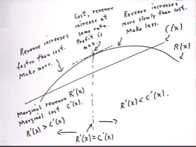
The rate at which revenue changes is R ' (x) and the rate at which cost changes is C ' (x). These quantities are called the marginal cost and the marginal revenue.
If we multiply R ' (x) by a small number of additional items we find the approximate corresponding increase in revenue.
If we multiply C ' (x) by a small number of additional items we find the approximate corresponding increase in cost.
That is, we multiply marginal revenue or marginal cost by a small number of additional items to find the approximate change in revenue or cost.
Note that the calculations here are R ' (x) * `dx, which is a differential approximation to `dR, and C ' (x) * `dx, which is a differential approximation to `dC..
Profit is maximized when marginal cost and marginal revenue are equal (i.e., slopes of R vs. x and C vs. x graphs are equal).