Class Notes

Analyzing Depth vs. Clock Time Data

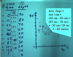
Given a set of depth vs. clock time data we can calculate average rates of depth change between every pair of successive clock times. If we hypothesize a quadratic model we can choose three points on our approximate 'best-fit' curve to use to create a model function y = a t^2 + b t + c. Substituting the y and t coordinates of our three points we obtain linear three equations in a, b and c, which can be solved simultaneously for these parameters. This will give us our model.

Solving the Equations

We solve the simultaneous equations by the process of elimination.

Using the Model

We can use the model to predict depth at a given clock time or to find clock time at which a given depth occurs.

Please Note:  The depth vs. clock time experiment is done in more detail in Precalculus I.  You may go to the Precalculus I homepage and see those details if you are rusty; however, knowledge of the quadratic formula, solutions of simultaneous equations, etc., should be very familiar to you, or should at least be something you can refresh without much trouble, as you enter a Calculus course.  Most Calculus students can refresh themselves from the level of detail provided here.

Analyzing Depth vs. Clock Time Data

Depth vs. clock time data are taken for water flowing from a uniform cylinder.   The depth vs. time data are plotted, yielding a graph which, as expected, falls less and less rapidly as time goes on.

• The average rate at which depth changes over each interval is easily calculated (middle column, showing `dy / `dt) by dividing the change in depth by the time required. 
• The result is the average rate for each time interval, in cm / sec.

• The average rate could also be calculated between any other pair of data points.  

• For example, during the 29 seconds between clock times 34 sec and 63 sec the depth changed by -20 cm, so the average rate was -20 cm / 29 sec = -.69 cm / sec.

• We note that this average rate is easily represented as the slope of the segment between the points (34 sec, 60 cm) and (63 sec, 40 cm). 
• The rise between these points is 40 cm - 60 cm = -20 cm, and the run is 63 sec - 34 sec = 29 sec. 
• The rise and run are shown as legs of a triangle, with the sloping segment between the points as the hypotenuse.

We arbitrarily chose the fourth, fifth and seventh points of the data set to use to obtain a quadratic model of the data. 

• These aren't the best possible points to choose--in fact, choosing three points isn't the way to get the most accurate quadratic model.  But the process is valuable because we will get a reasonably good model, and we will review some important mathematical techniques in the process.

• We plug the three data points, each with a value of y and a value of t, into the form y = a t^2 + b t + c. 
• We obtain three simultaneous linear equations, which we will solve by the standard technique of eliminating variables then back-substituting.

Solving the Equations

We choose first to eliminate c, since subtracting any equation from any other will eliminate this parameter. 

• We obtain two equations in the two unknowns a and b.
• Then we add appropriate multiples of these equations to eliminate b, obtaining an equation which we solve for a.

We substitute a into one of the equations for a and b, then solve for b; and we finally substitute our values of a and b into one of the original equations to obtain a, b and c.

Substituting the parameters yields the function model:

Using the Model

We can use this function model to predict the depth at any desired clock time, or the clock time at which any desired depth is attained.

For example to obtain the clock time t when the depth reaches 0, we let the depth y be zero:

• y = .00230 t^2 - .903 t + 88 so if y = 0

• 0 = .00230 t^2 - .903 t + 88 and, by the quadratic formula,

• t = [ -(-.903) + - `sqrt ((-.903) ^ 2 - 4 (.00230)(88) ] / (2 * .00230)

• (The rest of the solution is straightforward; however, we don't yet know whether the discriminant, the quantity we take the square root of, is positive, negative or zero.  

• If the discriminant is positive, we have two solutions, only one of which corresponds to reality.  
• If the discriminant is negative, we have no solutions, which can happen since our model is only approximate and needn't quite reach zero. 
• If the discriminant is zero, this is what we expect to happen in reality, but we're very surprised because our model is only approximate and the likelihood of an approximate model bottoming out at exactly zero is very small.)

To find the clock time when depth is 55 cm, we let depth y be 55:

• y = .00230 t^2 - .903 t + 88 so if y = 55

• 55 = .00230 t^2 - .903 t + 88.  We have to have zero on one side to use the quadratic formula, so we subtract 55:
• 0 = .00230 t^2 - .903 t + 33 and, by the quadratic formula,
• t = [ -(-.903) + - `sqrt ((-.903) ^ 2 - 4 (.00230)(33) ] / (2 * .00230).

• This time we obtain two solutions.  Our data shows us that y = 55 somewhere between 34 and 48 sec, so we accept the solution in this range and reject the other.

To find the predicted depth at clock time t = 0, we substitute t = 0:

• y = .00230 (0)^2 - .903 (0) + 88 = 88.

• Our prediction is y = 88 cm at t = 0. 
• Compare this with the data point (0,90).   88 cm is pretty close to the 90 cm we observed, so our model works pretty well for t = 0.

For t = 100 sec the predicted depth will be

• y = .00230 (100)^2 - .903 (100) + 88 = 20.7 cm.

• Our data set has y = 20 cm when t = 101 sec, so our prediction is pretty close here also.

To see how well our data fits, we could compare the prediction of our model with the data set for every time on the data set.  We would probably find that our model predicts the depth within a centimeter or two for every data point.  This is pretty good.

Further questions:

What does our function model tell us about the rates at which the depth changes?

How might we obtain a more accurate model?

How closely can we model this data with a quadratic function, anyway?