derivative and integral; numerical approximation of integral

Class Notes Calculus I

The Concepts of Differentiation and Integration in the Context of Rate Functions

Depth and Rate-of-Depth-Change Functions

The quadratic depth function y = a t^2 + b t + c implies a linear rate-of -depth-change function y ' = 2 a t + b. A linear rate-of-depth-change function y ' = m t + d implies a quadratic depth function y = 1/2 m t^2 + d t + c, where c is an arbitrary constant number while m and d are known if y ' is known. Thus the rate-of-depth-change function allows us to determine the change in depth between any two clock times; however to find the absolute depth at a clock time we must evaluate arbitrary constant c, which we can do if we know the depth at a given clock time.

The process of obtaining a rate function from a quantity function is called differentiation, and the rate function is called the derivative of the quantity function. The process of obtain the change-of-quantity function is called integration, and the quantity function is called the antiderivative or integral of the rate function.

Solution of Homework Problem from Modeling Project #2: Number of Decays obtained from Rate of Decay Function

From the function giving the rate at which a radioactive substance decays we estimate the number of decays over a substantial time interval. The process is depicted using a trapezoidal approximation graph.

Depth and Rate-of-Depth-Change Functions

To summarize the process of finding the derivative of a quadratic function, we begin by recalling that the idea of the derivative was introduced as a way to find the rate at which the depth of water in a uniform cylinder changes.

The average rate between two clock times was seen to be the corresponding depth change divided by the change in the clock time; the instantaneous rate was seen to be a limit as the time interval between the two clock time approaches 0.

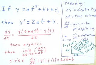
More specifically, if depth y is a function of clock time t, we could write depth = y(t).
In this case, between clock times t and t + `dt the change in depth is `dy = y(t + `dt) - y(t) and the change in clock time is `dt.
The average rate of change is then `dy / `dt = [ y(t + `dt) - y(t)] / `dt.
If the depth is a quadratic function of clock time, then for the appropriate values of parameters a, b and c, y(t) = a t² + b t + c.

When we use the quadratic function y = a t² + b t + c in the above process, we obtain `dy / `dt = 2 a t + b + a `dt.

The limiting value of this expression, as the time interval `dt approaches 0, is simply dy / dt = 2 a t + b.

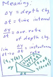
The figure below summarizes the meanings of the basic quantities used in the above calculation.

The graph near the bottom shows how the calculation of an average rate is equivalent to the calculation of the slope between the two points (t, y(t)) and (t + `dt, y(t + `dt)) on a graph of position vs. clock time.

video clip #21

http://youtu.be/joNdz_z8lTg

So we see that the quadratic depth function y(t) = a t² + b t + c implies the linear rate of change function y'(t) = 2 a t + b.

This means that we now have a formula for the rate of change function associated with a given quadratic depth function.

We now consider what we can conclude from a linear rate function y'(t) = m t + b.

Would a linear rate function necessarily be associated with a quadratic depth function?
We will prove later that this is the case.
For now we will be content to simply find this quadratic function.

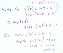
The figure below shows that if there is a quadratic depth function y(t) = a t² + b t + c, then since its associated rate function is y'(t) = 2 a t + b, this function is equivalent to the given function y'(t) = m t + b.

Since 2 a t + b = m t + b for all values of t, the parameter b is identical in both equations, while the coefficients 2 a and m of the variable t must be equal.
If 2a = m, then a = m/2, and are depth function must therefore be y(t) = .5 m t² + bt + c.

In other words,

Whatever the coefficient of the variable t in a linear rate function, the coefficient of the t² term in the depth function will be half as great.
Whatever the constant term in the linear rate function, the coefficient of t in the depth function will be equal to that term.

We note that this process tells us nothing of the c term in the depth model.

As stated in previous lectures, c can be any constant, unchanging number, which depends only on when we start our clock and position from which the depth is measured.

As an example, the rate function y'(t) = 5t - 3 is associated with quadratic depth function y(t) = 2.5 t² - 3 t + c

Note that the coefficient of t² in the depth function is identical to the coefficient of t in the rate function, and that the coefficient of t in the depth function is the constant term in the rate function.
To check we could find the rate function associated with this depth function, using the formula y'(t) = 2 a t + b.

video clip #22

http://youtu.be/_TQarfzPd6Q

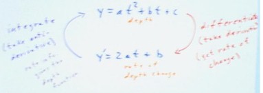
The figure below depicts the fact that the quadratic depth function implies a linear rate of change function (red arrow) and that the linear rate of change function implies a quadratic depth function (blue arrow).

The two figures below depict the meanings of the terms integration, differentiation and antiderivative:

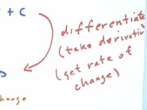
The first figure is a closer look at the right-hand side of the above figure, indicating that the process of finding the y'(t) function from the y(t) function is called differentiation, the process of taking the derivative to get the rate of change function.

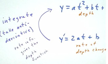
The second figure below depicts the left-hand side of the picture, indicating that when we reverse the process of differentiation we are said to integrate the rate of depth change function, obtaining a depth function.

When we do this we say that we are finding an antiderivative of the rate function.
We say that the rate information is integrated in order to find a depth function. (We say 'a depth function' rather than 'the depth function' because the parameter c is not specified and could therefore take any value).

video clip #23

http://youtu.be/4lq8WG02JpQ

These processes, differentiation and integration, are the two fundamental processes of calculus.

The Fundamental Theorem of Calculus, without which our technological civilization almost certainly would not exist in anything like its present form, essentially says that if we start with a rate function and integrate it we end up with a function whose derivative is the original rate function.

Once understood, this statement seems almost obvious in the context of depth models and rate functions. However it will later require some rigorous proof. And no matter how obvious it may eventually come to seem, its discovery was an act of genius perhaps unparalleled in human history.

video clip #24

http://youtu.be/sDrfPloQM4k

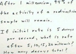
Solution of Homework Problem from Modeling Project #2: Number of Decays obtained from Rate of Decay Function

In the introduction to exponential functions, it was hypothesized that a certain radioactive substance would after one millennium (note missspelling of the word ' millennium') have 94% of its original activity.

The problem asks, assuming that the original rate at which the substance decays is 5 decays per second, what the decay rates should be after 5, 10, 15 and 20 millennia.
It furthermore asks what the approximate total number of decays during the 20 millennia should be.

If we let t be the clock time, in millennia, then every change of 1 in clock time t will reduce the activity to 94 percent of its former value.

The situation thus corresponds to an exponential decay with growth rate .94.
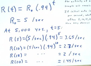
The corresponding exponential function giving rate as a function of time would be R(t) = R0 (.94) ^ t.
The initial rate R0 is the 5 decays per second specified in the problem.

We see this function evaluated at R = 5, 10, 15 and 20, corresponding to the 5, 10, 15 and 20 millennia of the original problem.

We obtain the rates 3.65, 2.7, 2, and 1.45 decays/second (apologies with regard to inconsistency in the significant figures).

video clip #25

http://youtu.be/xZDtpDMYrgo

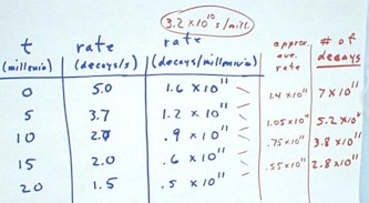
These results are summarized in the first two columns of the table below.

In order to answer the question of how many decays occur over the 20 millennia, the decay rates are translated in the third column to decays per millennium.
The conversion factor 3.2 * 10 ^ 11 seconds / millenium is shown above this column, and results have been rounded to the nearest .1 * 10 ^ 11 decays/millennium.

The fourth column shows the approximate average rate at which the substance decays over each of the four time intervals between zero and 20 millennia.

In each case the approximate average rate is obtained by averaging the rate at the beginning at the end of the time interval.
No matter how precise our figures, note that this average will give only an approximate average rate, since when we average the two rates we implicitly assume that the rate changes in a linear fashion; the actual case for an exponential function is that the rate goes down at a constantly changing rate and is not linear. (Once more note that liberties have been taken with the number of significant figures, and that this affects the reliability of the final results).

In the fifth column the average rates, in decays/millennium, are used to find the approximate total number of decays during the 5 millennia of each time interval.

video clip #26

http://youtu.be/wGmrNQLtURU

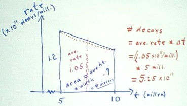
The figure below shows the calculation of the number of the decays during the second 5-millenium period. Note that the result in the table has been incorrectly rounded to 5.2 rather than 5.3 decays.

We depict the process graphically by a trapezoid on a rate vs. clock time graph.

During the second millenium we see that the rate decreases from 1.2 to .9 (both x 10^11) decays / millenium.
These quantites are depicted by the vertical sides of the trapezoid, since rate is measured in the vertical direction.
If the rate changes at a constant rate, the graph will match the sloping top of the trapezoid.

However, since in this case the exponential function has a curve, as depicted by the dotted red line on the graph, we are only approximating the real behavior of the function.

We see that because the interval is fairly small, our approximation is never very far from the actual function.

The average rate over the time interval from 5 to 10 millenia is then approximately equal to the average of the 1.2 * 10 ^ 11 and .9 * 10^11 decays / millenium, or 1.05 * 10^11 decays / millenium.

This average corresponds to the midpoint altitude of the trapezoid.

To get the number of decays, we multiply the average rate by the duration of the time interval, in this case multiplying 1.05 * 10^11 decays / millenium by the 5 millenia of the time interval, to get 7.25 * 10^11 decays.

In multiplying the average rate by the time interval, it should be clear that we have multiplied the average altitude of the trapezoid by its width.
We have therefore calculated the total area of the trapezoid, and see that the area of this trapezoid corresponds to the number of decays over the corresponding time interval.

video clip #27

http://youtu.be/jKUoHwBaLko

In the above process we have taken rate information and obtained information about the original quantity, in a manner completely analogous to what we might have done in order to find depth changes from rate of depth change information.

In both cases we multiplied the approximate average rate by a time interval in order to get the change in the quantity.

The quantity in this case is the number of decays, while in the original example it is the number of cm of depth change.

Again, this process of obtaining the change in quantity from the rate information is called integration.

In the present example we did a numerical approximation to find the change in quantity (the number of decays).
We therefore call this process 'numerical integration'.

If we knew the rule for taking the derivative on exponential function, we could do as we did with the depth vs. time model and find from the given rate function the function that gives us the total number of decays as a function of time.

Later in the course we will develop the rules for differentiating and integrating exponential functions.

video clip #28

http://youtu.be/0McQXGge8H0