Class Notes

Class Notes Calculus I

Growth of an Exponential Function; Trapezoidal Representation of Approximate Derivatives and Integrals

Growth Rate, Growth Factor and the Quantity Function; Doubling Time

An exponential function is characterized by a growth rate r, a growth factor (1+r) and a quantity function Q(t) = Q0 (1+r)^t. Alternative forms of the exponential function include Q(t) = Q0 b^t and Q(t) = Q0 e^(kt).

Any function of this form has a doubling time tD such that for any t, Q(t+tD) = 2 Q(t), which we demonstrate algebraically and depict graphically.

Representation by and Interpretation of Trapezoids

Given a velocity vs. clock time function we can construct a trapezoid between any two graph points, with vertical altitudes running from the horizontal axis to the respective graph points. These altitudes represent the initial and final velocities over the corresponding time interval. The area of this trapezoid represents the product of the average of the initial and final velocities and the duration of the time interval, and therefore the distance that an object would move during the time interval at this average velocity. If the velocity function is not linear during time interval, it is very unlikely that the actual average velocity will equal the average of the initial and final velocities, and the distance so calculated will be an approximation rather than a precise value. The slope of the line segment between the graph points will represent the average rate at which the velocity changes (change in velocity divided by change in clock time).

In general if the graph represents the rate at which some quantity changes vs. clock time, a trapezoid can be constructed to approximate the change in the quantity between to given clock times, with the change in the quantity represented by the area of the trapezoid. More accurate approximations can be obtained by subdividing the trapezoid into a series of 'thinner' trapezoids, on which the line segments between graph points more nearly approximate the actual function.

The area under the graph between two clock time therefore represents the integral of the rate function between the two clock times. This integral represents the change in the quantity between these two clock time.

If the graph represents some quantity vs. clock time, then a similar trapezoid or series of trapezoids will have line segments between graph points which represent average slope between graph points, and which therefore represent average rates of change between the corresponding clock times. These average rates of change represent the approximate derivatives of the function depicted by the graph.

If the clock times on a series of trapezoids are uniformly spaced, then if the slopes represent rates of change, then at any graph point the change in slope at that point divided by the uniform time interval between graph points will represent the approximate rate at which the slope changes at the graph point. Since the slope represents the rate at which the function changes, this rate of slope change will represent the rate at which the rate changes. This quantity is and approximate second derivative of the function.

By interpreting the altitude and width of a trapezoid, we can interpret what the product of average altitude and width represents, and we can interpret what is represented by the change in altitude divided by the width.

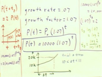
Growth Rate, Growth Factor and the Quantity Function; Doubling Time

If $10,000 is invested at 7%, compounded annually, and if at some instant we have principle P, a year later we will have 7% more than P.

This means we will have P + .07 P, or 1.07 P.

We call .07 the growth rate. Since we multiply by 1.07 in order to get the principle a year later, we call 1.07 the growth factor (recall that a factor is a quantity that is multiplied by another quantity).

To find the principle t years after the instant the principle is P, we first multiply by 1.07 to get the principle after one year, then we multiply this by 1.07 to get the principle after another, then by 1.07 to get the principle after still another year, etc., until we have multiplied by the growth factor 1.07 total of t times, once for each year.
The result of this process, multiplying an original principle by 1.07 total of t times, is to multiply the original principle by (1.07) ^ t.
If our original principle, at t = 0, is P0, then after t years the principle will be P0 * 1.07 ^ t.
Thus our principle is modeled by the function is P(t) = P0 (1.07) ^ t.
In the present case original principle is P0 = $10,000, so we have P(t) = $10,000 (1.07) ^ t.

In order to estimate the time required to double the principle to $20,000, we could sketch the 'green' graph below, showing principle that starts at $10,000 and increases along the exponential curve to $20,000.

The time interval `dt can be determined by trial and error, plugging different t values into P(t) until we reach $20,000.
The result of this trial and error is an approximation to `dt; `dt will lie between 10 and 11 years.

Video clip #41

http://youtu.be/DcfTpzvX-TM

It turns out that this doubling time is independent of the time when we begin.

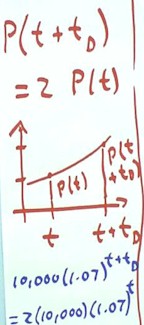
If t stands for an arbitrary time and t_D for the time required to double, then we start with principle P(t) at time t, and after the passage of time t_D, when the time is t + t_D, we have double this principle.
This situation is described by the equation P(t + t_D) = 2 P(t), written above the 'red' graph below.

The graph depicts this situation, in which P(t) is seen to double between time t and time t + t_D.

Since P(t+t_D) = $10,000 (1.07) ^ (t + t_D) and P(t) = $10,000 (1.07) ^ t, our equation becomes

10,000 (1.07) ^ (t + t_D) = 10,000 (1.07) ^ t.

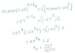
We can solve this equation by noting that 1.07 ^ (t + t_D) = 1.07 ^ t * 1.07 ^ t_D.

We first divide by the 10,000, then we express 1.07 ^ (t + t_D) as specified and divide by 1.07 to obtain the equation 1.07 ^ t_D = 2.

You are not required to know how to use logarithms to solve the equation at this point, but you should have encountered this process in your prerequisite courses, and you should get used to the remaining steps.

We begin by taking the logarithm of both sides of the equation.

Since a basic rule logarithms is log(a^b) = a log(b), log(1.07 ^ t_D) = t_D log(1.07) and we have t_D log(1.07) = log(2).

We easily solve this equation to determine that t_D = log(2) / log(1.07); this exact result can be approximated by your calculator.

Video clip #42

http://youtu.be/VloWD-snmVg

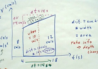
Representation by and Interpretation of Trapezoids

Suppose that, between clock times t = 4 sec and t = 18 sec the velocity of an object increases from 8 cm per second to 12 cm per second.

We can represent the situation by the graph shown above.
The sloping line at the top of the trapezoid represents velocity increasing linearly from 8 cm per second to 12 cm per second.
We don't know for sure that the increase is linear, but in the absence of information to the contrary, we make this assumption and recognize that our results will be approximate.

We are interested in two quantities, the area and the slope of the trapezoid.

The area of the trapezoid is equal to its average altitude multiplied by its width.
Since the altitude goes from 8 cm per second to 12 cm per second, the average altitude is 10 cm/s.
Since the altitudes represent velocities, the average altitude represents the average velocity.
The width of the trapezoid goes from t = 4 s to t = 18 s, so the width is 14 seconds.
This width therefore represents a time interval, over which the velocity averages 10 cm per second.

When we multiply the average height by the width, we multiply 10 cm per second by 14 seconds and obtain 140 cm.
Since we multiplied average velocity by the time over which the velocity has been average, we have obtained the change in our position, which is the distance moved.

Thus the area of a trapezoid on a velocity vs. clock time graph will give us the change in position of the object whose velocity we are representing.

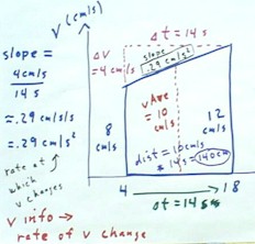
The slope of the trapezoid, by which we mean the slope of the line at the top of the trapezoid, is easily found by dividing the 4 cm rise by the 14 second run to get .29 cm/s/s.

We have divided the change in velocity by the time over which the change occurs.
This gives us the average rate at which velocity changes.
In this case the rate is.29 cm/s/s, which tells us that on the average, every second the velocity changes by.29 cm/s.
The quantity .29 cm/s/s, the average rate in which velocity changes, is called the average acceleration.

Note that the velocity is the rate which position changes, and the area gives us the change in the position between the two specified clock times.

More generally, we see that the area of a rate vs. clock time graph represents the change in the quantity whose rate is given.

So the process of calculating trapezoid areas uses rate information and gives us change in quantity.

In the same way we have used rate of depth change information to obtain the depth change between two given times.

We note also that if we regard the velocity as a quantity, the slope of the graph gives us the average rate which that quantity changes.

So the process of calculating trapezoid slopes takes our information about quantity and translates it into the rate of change of that quantity.
In the same way we have used depth information to obtain the rate which depth changes.
This is the process we have called 'differentiation', the finding of derivatives.

Recall that the derivative of a quadratic depth function y = a t^2 + b t + c is y' = 2 a t + b, giving us the instantaneous rate at any clock time.

Recall the the preceding process, in which we calculated the area under the graph, is called integration.

We originally used integration to find the depth change from the rate of depth change function.

Recall that the integral of a linear rate function y' = mt + b is y = .5 m t^2 + bt + c, from which we can find the depth change between any two clock times.

Video clip #43

http://youtu.be/N5BSn5TIprw

Video clip #44

http://youtu.be/fBJO0fZs5Y4

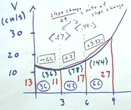
For practice suppose that we have a quadratic velocity vs. clock time function whose values at t = 0, 3, 6, and 9 sec were 13, 11, 17 and 27, respectively.

These values of the velocity are depicted in red, and the red trapezoids depict the approximation we obtain if we assume the linear velocity change between each pair of points.

Note that the quadratic fit to the first, second and fourth points tells us that the third point should have v = 15 2/3 rather than 17, so the data we have represented isn't perfectly quadratic.

We easily calculate the area under each trapezoid.

These areas are circled within each trapezoid and represent the 36 meter approximate change in position, or distance traveled, during the first three seconds, the 42 meter approximate distance traveled during the next three seconds, and the 66 meters traveled during the last three seconds.
The total approximate distance up to the 3 second clock time is therefore 36 meters.
The total approximate distance up to the 6 second clock time is obtained by adding the 42 meters traveled during the second time interval, to obtain 78 meters.
To this we add the 66 meters traveled during the last time interval to obtain a total distance of 144 meters.
These 'accumulated areas' are represented by numbers in parentheses within each trapezoid.

Note that these distances are all approximations based on the assumption of straight-line approximations to the curved graph.

It is evident from the graph that these approximations are all a bit high, since the trapezoids uniformly lie slightly above the curve.

Video clip #45

http://youtu.be/e9BC6ego_io

The slopes are also easily calculated, and each slope represents the average rate at which the velocity changes between two graph points.

The slopes are labeled by numbers above the top of the trapezoid, which are enclosed in a rectangle to indicate fact that they represent slopes and not lengths.

We note that at t = 3, the slope changes from -.66 to +2.

We therefore say that the slope change at clock time t = 3 is the increase 2.66 from the former to the latter slope.
This increase was based on consistent time interval of `dt = 3 seconds, so we say that the approximate rate at which slope changes at clock time t = 3 is 2.66 / 3 = .87.

We indicate this by the <.87> label above the t = 3 point on graph.

We similarly note that the slope change is 1.33 at the t = 6 point, so that the average rate at which the slope changes at that point is 1.33 / 3 = .44.

This is indicated by the <.44> above the t = 6 graph point.

Video clip #46

http://youtu.be/WNCJXV7Cyl4

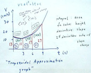
All these quantities are arrived at by trapezoid approximations of the actual graph. We therefore call this graph a "trapezoidal approximation graph".

On such a graph the value of the function is represented by the height of the graph, which is labeled next at a vertical line representing this value and forming a side of a trapezoid.

The area of the graph is interpreted as the change in the quantity whose rate is represented by the height.

Areas are added up into a total area which represents the approximate integral of the function over the range of t values represented by the graph.

We call this quantity an integral because it is obtained by integrating (making into one) the areas of a number of approximate in trapezoids.

The slopes of the graph are interpreted as the average rates of change of the quantity represented by the height.

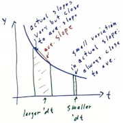
If on a y vs. t graph the time increments represented by the trapezoids are small, the slopes are close to the limiting values of `dy / `dt as `dt shrinks toward zero.

These slopes are therefore approximate derivatives.

When we calculate the rates at which slopes change, we are calculating the approximate derivatives of the slope.

Since the slope itself is the derivative of the quantity represented on the vertical axis, the rates which the slopes change represent approximate derivatives of derivatives.
We call such quantities approximate second derivatives.

Video clip #47

http://youtu.be/8EkHv2vccEI

The graph below represents the same curve between the same two points, approximated by a larger number of trapezoids.

On this graph the time interval `dt is much smaller than before.
We note that the sloping 'tops' of these trapezoids stay much, much closer to the curve than before.
In fact, though we have used only about 4 times as many trapezoids as before, we are on the average much better than 4 times closer to the actual function than we were before.

Thus our slopes, and hence our rate of change approximations, are much much closer to the actual instantaneous rates of change of the function.

Similarly our total area, hence our approximation of the change in quantity, is much much closer to the actual area than before.

We can imagine shrinking the time interval `dt to 0.

Our approximations will become dramatically better with every decrease in `dt, and rapidly approach the precise instantaneous slopes or rates of change, and the precise areas under the graph.

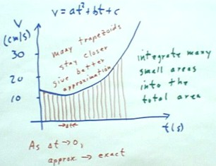
Video clip #48

http://youtu.be/VWcJinRJlig

This picture is related to the work we have done to find the derivative of a quadratic function as follows:

If the graph is of the function y = a t^2 + b t + c, then as we have seen, at any clock time t the instantaneous rate which the function is changing is y' = 2 a t + b.

If we have a trapezoidal approximation graph, it follows that if t is any specific clock time within the range represented by the graph, t lies in one of the intervals.

This interval defines a trapezoid with a slope m.

To the extent that the time intervals are short, m will therefore be close to the instantaneous slope y' = 2 a t + b.

Though we have not yet developed the means to determine the precise total area under a quadratic graph, or the integral of a quadratic function between two given points, it turns out that the area, from t = 0 to given value of t, is

precise area = a t^3 / 3 + b t^2 / 2 + c t.

As `dt -> 0, the total area as calculated by the trapezoidal approximation will approach this value.

If we have the graph of a linear function y = m t + b, we can easily calculate its area between the points (0, b) and (t, mt + b):

The time interval is `dt = t - 0 = t, and the average altitude is the average of the two altitudes m and mt + b, or (b + (mt + b) ) / 2 = .5 m t + b.

The area is thus the product of the average altitude and the width, or area = (.5 m t + b) * t = .5 m t^2 + b t.

This is a quadratic function of clock time, and corresponds to the .5 m t^2 + b t + c function we obtained earlier as the integral of y' = m t + b (in this specific case we have for the unspecified parameter c the value c = 0).

Note that this area function is a quadratic function with a = .5 m and b = b, so that its derivative is 2 a t + b = 2 (.5m) t + b = mt + b.

Video clip #49

Examples of interpretation:

If we graph population of a species in an ecosystem vs. clock time (we imagine a very slow clock that runs in weeks or years or whenever unit is appropriate to the species), then the altitude, or vertical coordinate, of a graph represents the population and the horizontal quartet represents the clock time.

The slope of such a graph will therefore represent the change in population divided by the time interval over which the change occurs.

This gives us the rate of which population is changing.

If we graph the rate at which a plant is gaining mass, in grams / day, vs. the clock time t, then the area under the graph between two clock times will represent the product of the average altitude of the graph multiplied by the average width.

The average altitude of the graph will represent the average rate at which mass is gained, and the width will represent the length of the time interval over which this average applies.

The product will therefore represent the gain in mass.