"
Class Notes Calculus I
Interpretation of the Derivative; the Second Derivative; Area under a
Curve; Right- and Left-Hand Sums
The quiz problem stated that a function y = f(t) gives the expected grade point average
for t, the number of hours per week of study.
- The question was to interpret the statements
- f(30) = 3.6,
- f ' (12) = .16 and
- f ' (25) = .03,
- and then to estimate the expected increase in grade point average for someone who is
currently spending 12 hrs / wk studying.
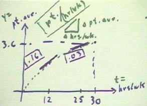
The graph below depicts the given information.
- f(30) = 3.6 implies the point (30, 3.6), as indicated by the projection lines.
- f ' (12) = .16 is the rate of change, or slope, at the t = 12 point of the graph.
- It is not clear just what the graph looks like, but the fact that f ' (12) = .16 while f
' (25) = .03 implies that the slope might be decreasing; the green dotted line represents
a graph with decreasing slope that passes through the known point (30,3.6). (Note that
from knowledge of the derivative function and the known point we could in fact construct
the function f(x) by a process of integration, in the process solving a differential
equation).

We interpret the statement f ' (12) = .16 to indicate that for someone studying 12
hours per week, for every unit of run (corresponding to every hour of increased study
time) there will be a .16 unit of rise (corresponding to an increase of .16 in point
average).
- The rate of change therefore gives the increase in grade point per hour of additional
study time.
- Similarly the statement f ' (25) = .03 indicates that for someone studying 25 hours per
week, the expected grade point will go up by .03 per additional hour of study time.
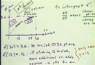
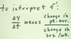
In general, `dy / `dt stands for the change in point average divided by the change in
the hours per week of study time.
Video Clip #1
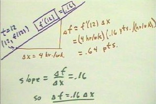
If an individual studying 12 hours per week increases study time by four hours per
week, the situation corresponds to the graph shown below.
- The point (12, f(12)) gives the x and y coordinates of the graph for t = 12; f(12) is
not known, so cannot be given any more specifically.
- The rate of change f ' (12) = .16 points / (hr / wk), is the slope of the graph at that
point. Beyond that point, the slope probably decreases, and the point average goes up less
quickly.
If the rate did stay the same, then an increase of 4 hrs / wk would imply an increase
in point average of 4 * .16 points = .64 points.
- This should be obvious, but it
doesn't hurt to depict the situation in symbols.
- The additional four hours per week
is a change `dx in the independent variable x, and we are looking for the change in the
dependent variable y = f(x); we denote this change by `df.
- The slope is then slope = `df /
`dx = .16, so `df = .16 * `dx = .64.
Video Clip #2
The Second Derivative
As we will see, since the derivative of function is rate at which the function changes,
the derivative of the derivative is the rate at which the rate changes.
- The derivative of the derivative of a function is called the second derivative
of that function.
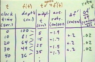
We begin with a table of depth vs. clock time for a hypothetical flow from the uniform
cylinder.
- As we have seen the depth vs. time function seems to be quadratic.
- The f(t) vs. t data shown below are in fact quadratic.
To obtain a table of approximate values for the rate function, we first calculate the
midpoint of each time interval; the average rate over an interval will be associated with
the midpoint clock time..
- The time intervals are defined by
the clock times 0, 10,20, 30 and 40 seconds.
- The midpoint times are therefore
5,15, 25, and 35 seconds.
We calculate the average rate at
which depth changes over each interval, and associate this average rate with the midpoint
time.
- In general this gives us only an
approximation of the rate function, but for a quadratic function the values we get are in
fact accurate.
Video Clip #3
The third and fourth columns of the table therefore give us approximate (and in this
case accurate) values for the derivative function f ' (t) vs. t.
We now wish to determine the average rates at which this derivative function
changes.
- The first thing we probably notice about the derivative function is that it appears to
change a constant rate, changing by .2 cm/sec during every 10 second interval.
- This will not always be the case, of course, since we will not always be dealing with
quadratic functions.
- We therefore proceed to make a column for the changes `df ' in the derivative
function.
- These changes are, as observed, always +.2 cm / sec.
- We then divide the `df ' values by the 10 second time interval to obtain the
average rates at which the function changes.
- In this case every rate turns out to be .2 cm/sec / (10 sec) = .02 cm / sec / sec.
The rates we have just calculated is the rates at which the rate f ' (t) changes.
- So we have values for the depth
function y = f(t), the rate of depth change function f ' (t), and the (constant in this
case) rate at which the rate of depth change changes.
- This last rate is a limit of the
average rate `df ' / `dt at which f ' changes.
- When we take the limit of `df '
/ `dt as `dt -> 0, we obtain the derivative of f ' , which we designate (f ' )'
or simply f ' '.
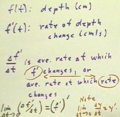
To be sure we understand this notation, we note that lim (`dt -> 0) (`dy / `dt) =
y'.
- If we then substitute f '
for y, we see that y' = (f ' )'.

Video Clip #4
We can obtain another picture of the rate which the depth changes by considering a
trapezoidal approximation graph of some function.
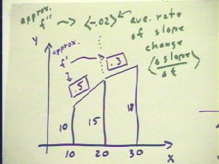
- The figure below shows such a graph.
- We understand that y represents a function f(x), and we see from the graph that the
values of the function for x = 10, 20 and 30 are 10, 15 and 18.
- The slopes associated with the resulting trapezoidal approximation are .5 and .3, and
indicate approximate values of the derivative function f ' .
- Without further knowledge of the behavior of the function, we choose to associate these
average values of f ' with the midpoint x values 15 and 25 for the two trapezoids.
These f ' values represent
average rates.
- We see that these average rates are changing and we can in fact see that over the
10-second interval (from midpoint x to midpoint x) the rate decreases from .5 to .3, a
change of -.2.
- To get the rate at which the rate changes, we have to divide this change by the 10-unit
interval over which it occurs.
- With thus get an average rate of rate change equal to -.02.
- We note that we can also think of this average rate at which the rate changes as the
average rate of which the slope changes; slope changes by -.2 over an interval of `dx =
10.
- By convention we represent this average rate of slope change as <-.02>, as
depicted in the figure below.
Video Clip #5
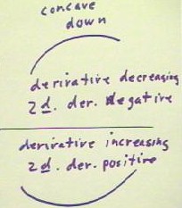
We observe that in the above figure the derivative is decreasing, which makes the graph
concave downward (if the graph forms a 'cave', then when we are sitting in the cave
looking at, we are looking out downward as opposed to upward).
- This will be the case any time the derivative is decreasing.
- As we have seen a decreasing derivative f ' implies a negative second derivative f
' '.
- So, as indicated in the figure below, a graph which is concave downward implies
a decreasing derivative and a negative second derivative.
Video Clip #6
Similarly a graph which is concave upward implies an increasing derivative and
hence a positive second derivative.
Recalling that a quadratic depth vs. clock time data set yields a constant rate of rate
change, implying a constant second derivative, we look at the second derivative of
a general quadratic function.
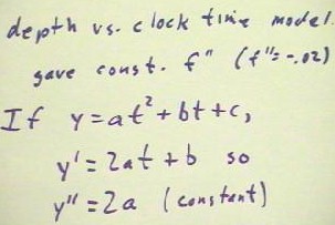
- The derivative of the function y = a t^2 + b t + c is y' = 2 a t + b, as we have seen.
- It is easy to see that the derivative of this function must be simply y'' = 2a.
- Since a is a constant number, y'' = 2a must also be a constant number.
- This proves what we have seen: that the slopes or rates of quadratic functions
change at a constant rate.
Video Clip #7
Area under a Curve
We now turn our attention to the interpretation and calculation of the area under a
curve.
We begin with an example of a velocity vs. clock time graph.
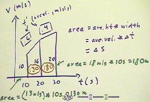
- The graph below depicts the velocity, in meters/second, of some object at clock times t
= 10, 20, and 30 seconds.
- We do a trapezoidal approximation of the function, based on the velocities 10, 16 and 20
m/s at these three clock times.
- We can of course calculate the slopes .6 and .4 and label these according to our
conventions; we can also interpret the slopes as the average rates and which velocity
changes over the two time intervals.
- We note this fact and then move on to the calculation and interpretation of the areas of
the two trapezoids.
- The area of the first trapezoid, equal to the product of its average height and its
width, is 13 * 10 = 130.
- The average altitude 13 represents the average 13 m/s of the two velocities 10 m/s and
16 m/s, and the width represents the 10 seconds over which this average velocity applies.
- Moving at 13 meters/second for 10 seconds gives us a displacement of 130 m.
- The area of any trapezoid on this graph will be calculated similarly, multiplying
average height by width and thereby representing a product of velocity in meters/second
and time interval in seconds.
- The area of the second trapezoid is easily found to be 180, representing the 180 meters
moved during the 10 second interval between clock times t = 20 and t = 30 seconds.
Video Clip #8
We note that the total distance traveled between clock times t = 10 and t = 30 sec is,
according to this graph, the sum 130 m + 180 m = 310 m of the distances represented by the
areas of the individual trapezoids.
- If this graph represents a trapezoidal approximation of some continuous function y =
f(t), then 310 is an approximation to the total area under the curve defined by the graph
of that function between the values t = 10 and t = 30.
- Had we used a greater number of trapezoids between these two t values, we would almost
certainly have remained closer to the actual curve of the function and obtained a more
accurate approximation of the precise area.
- We say 'almost certainly' because it is possible for some functions, especially some
cyclically varying functions, to make an unfortunate choice in the lengths of our
intervals and obtain a very poor approximation to the correct area.
We now show that for a function y = f(t) whose values are strictly increasing on an
interval between t = a and t = b, the area of the trapezoidal approximation in fact does
approach the precise area under the curve as the number of trapezoids approaches infinity.
- That it should be so might seem obvious, but as the exception noted at the end of the
preceding paragraph should indicate, we have to be very careful about things that seem
obvious. Our intuition can easily mislead us, and we need to find a precise mathematical
proof of what we think must be true before we really trust our inclinations.
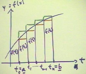
The graph below depicts a function y = f(t) between t values t = a and t = b.
- We imagine dividing the region under the graph into n segments defined by t values t0,
t1, t2, . . . , tn.
- Since the interval runs from t = a to t = b, the first value t0 must be equal to a, and
the last value tn must be equal to b.
- The two values of t following t0 are t1 and t2; the value preceding tn is t(n-1).
- We assume here that each interval of the t axis has the same width `dt.
The function values corresponding to these values of the independent variable t will
therefore be f(t0), f(t1), f(t2), . . . , f(t(n-1)) and f(tn).
- We note that since the function is strictly increasing, f(t0) < f(t1) < f(t2) <
... < f(t(n-1)) < f(tn).
Rather than doing a trapezoidal approximation, we do two approximations by rectangles,
called the 'upper sum' and the 'lower sum'..
Video Clip #9
Lower Sum: The first approximation will be a 'lower sum', where
for each interval we use the altitude at the left-hand side of the interval.
- Since the values of f(t) are strictly increasing, these left-hand altitudes will be the
minimum altitudes on the various intervals, and the resulting areas must therefore be less
than the corresponding areas under the actual curve.
- On the first interval the altitude will therefore be f(t0). Since the width `dt is the
same for all rectangles, the area of this first rectangle therefore be the product f(t0) *
`dt of its altitude and width.
- On the second interval the left-hand altitude will clearly be f(t1), so the area will be
f(t1) * `dt.
- On the third interval area will be f(t2) * `dt), and the progression will continue up to
the last interval.
- On the last interval the left-hand altitude will be based on t = t(n-1), so the area
will be f(t(n-1)) * `dt.
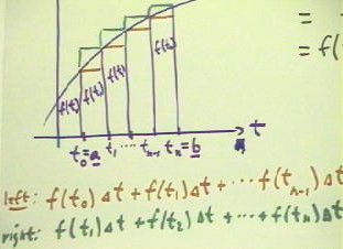
Our total left-hand, or 'lower' approximation of the area between t = a and t = b will
therefore be
- lower approximation = f(t0) * `dt + f(t1) * `dt + f(t2) * `dt + . . . + f(t(n-1)) * `dt.
This lower approximation will be the sum of the areas of all the rectangles bounded
above by the red segments in the figure below.
Upper Sum: The 'upper' sum will be obtained by using the
right-hand altitude of each segment.
- For the first segment the altitude is f(t1) and the areas therefore f(t1) * `dt.
- For the second and third segments the altitudes will be f(t2) * `dt and f(t3) * `dt.
- For the last segment will use the right-hand altitude f(tn), obtaining area f(tn) * `dt.
When we add all these areas we obtain the 'upper' approximation
- upper approximation = f(t1) * `dt + f(t2) * `dt + f(t3) * `dt + . . . + f(tn) * `dt.
We note first that the average of the upper and lower approximations will in fact give
us the trapezoidal approximation to the total area, since by averaging these
approximations we are in effect averaging the two altitudes of each trapezoid.
We then ask whether it must in fact be the case that as we allow the widths `dt to
approach 0, the difference between the upper and lower sums also approaches zero.
- If this is the case, then the total area under the curve must be 'squeezed'
between the sums and must therefore be equal to the limiting value of either sum.
The difference between the upper and lower sum will represent the total area of the
increasingly small rectangles defined by the red and green segments.
- If we imagine what happens when the interval `dt shrinks to zero, we will see that the
total area of these rectangles also shrinks rapidly, and we fully expect from this image
that their total area will shrink away toward zero.
- However, we recall that we must rigorously test our expectations to be sure that they
are valid.
If we look at the expressions for the right- and left-hand sums, we quickly see that
they both contain the term f(t1) * `dt.
- Similarly both sums must contain the terms f(t2) * `dt, f(t3) * `dt, . . . , f(t(n-1)) *
`dt.
- The only terms that are not shared are the f(t0) * `dt of the left-hand sum, which never
appears in the right-hand sum, and the f(tn) * `dt of the right-hand sum, which never
appears in the left-hand sum.
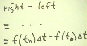
Thus, when the left-hand sum is subtracted from the right-hand sum, all the common
terms will be 'canceled' and we will be left with only f(tn) * `dt - f(t0) * `dt.
Video Clip #10
Since we originally assumed that f(a) = f(t0) and f(b) = f(tn) are finite numbers, it
follows that as `dt approaches 0, the expression f(tn) * `dt - f(t0) * `dt = (f(tn) -
f(t0)) * `dt must approach 0.
- This proves that, for any interval on which a function is strictly increasing and on
which the function is finite at both endpoints, the difference between the left-hand and
right-hand approximations approaches 0 as the number of equal increments into which the
interval is partitioned approaches infinity.
- This ensures us that the error of a trapezoidal approximation, which is clearly less
than that of the difference, also approaches 0 so that the trapezoidal approximation
approaches the actual area under the curve.
- Furthermore, since the area under the curve must lie between that of the left-and
right-hand approximations, in the limit either of these approximations must approach the
actual area under the curve.
"
