Calculus II Class 01/29
Calculus I Quiz 0129
Give all possible substitutions and all possible breakdowns into u and dv, then see which, if any, lead to a closed-form result for each of the following integrals:
integral ( t^4 ( 1 - t)^2 dt )
It is possible to break down this integrand into u and dv in many ways. It will however turn out that integration by parts is not the easiest way to perform this integral.
Possible breakdowns include:
u = t^4, dv = (1-t)^2 dt
u = t^3, dv = t ( 1-t)^2 dt
u = t^2, dv = t^2 ( 1-t)^2 dt
u = t, dv = t^3 ( 1-t)^2 dt
u = (1-t)^2, dv = t^4 dt
u = t (1-t)^2, dv = t^3 dt
u = t^2 (1-t)^2, dv = t^2 dt
u = t^3 (1-t)^2, dv = t dt
u = t^4 (1-t)^2, dv = dt
u = (1-t) , dv = t^4(1-t) dt
u = t(1-t) , dv = t^3(1-t) dt
etc.
In every case dv can be integrated and the integration by parts formula can be applied, and in every case if we are persistent we will more or less quickly arrive at a form in which we can evaluate the integral.
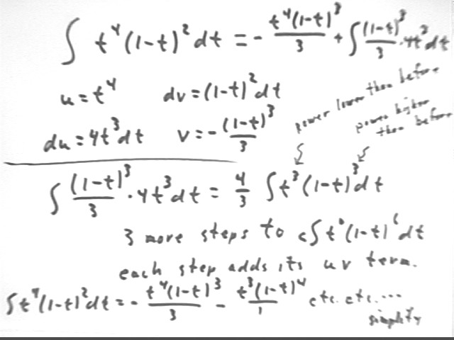
The figure below shows how this might work out for the breakdown u = t^4, dv = (1-t)^2 dt.
We note that an antiderivative of (1-t)^2 is -(1-t)^3 / 3.
On the first step we arrive an an integral which can be expressed as 4/3 integral ( t^3 ( 1-t)^3 dt).
We have succeeded in lowering the original t^4 to a multiple of t^3, which seems like progress.
We have however increased the power of (1-t) to 3, as opposed to the original power 2.
We could continue this strategy for 3 more steps, at each step decreasing the power of t and increasing the power of (1-t).
At each step our u v term will introduce an additional expression analogous to the -t^4 (1-t)^2 / 3.
The last integral we will encounter will be a multiple of the integral of t^0 * (1-t)^6, or just (1-t)^6, which will give us a multiple of (1-t)^7.
The result will be a mess, and we will need to expand all terms and the collect like terms.
Any of the breakdowns into u and dv will lead to a similar mess.
In every case the simplified form of the final expression will be the same.
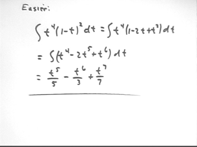
As we will see below, however, if we had just expanded the integrand in the first place we would have saved all this trouble.
The integrand is easily expanded into a simple polynomial, as shown below.
The result shown here is equal to the result that could have been obtained by the much messier process illustrated above.
The lesson is, if your integrand can be expanded in powers of t, do so and don't mess with substitutions and integration by parts.
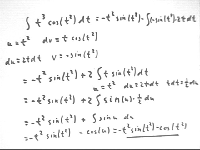
integral ( t^3 cos(t^2) dt)
This integral can be done using integration by parts. It can also be done by substitution, and a successful integration by parts will in fact rely on an equivalent substitution in order to integrate the factor dv.
We note in the figure below several possible breakdowns of the integrand into u and dv.
We note that dv = cos(t^2) dt and dv = t^2 cos(t^2) dt can't easily be integrated.
However we might recognize that dv = t cos(t^2) dt can be integrated using the substitution w = t^2, giving us v = 1/2 sin(t^2).
dv = t^2 dt and dv = t^3 dt will end up increasing the power of t in our integral, which probably isn't a good idea.
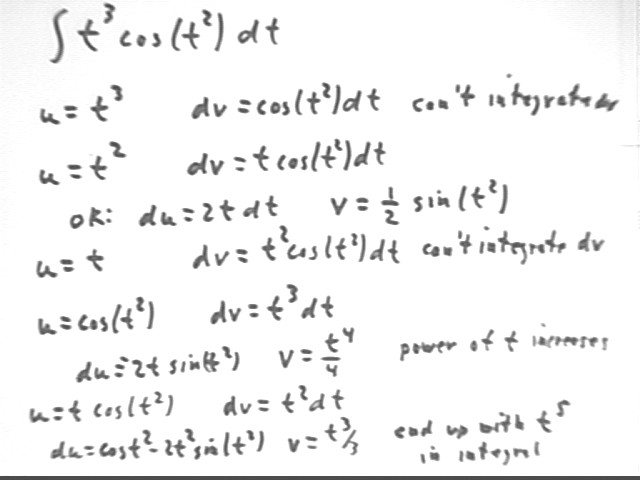
Below we use the breakdown u = t^2 and dv = t cos(t^2) to obtain our result.
We can easily validate the process by verifying that the derivative of -t^2 sin(t^2) - cos(t^2) is indeed equal to t^3 cos(t^2).
Look at the table of integrals in the back of your book. See if you can find the form corresponding to each of the following, and give the value of each of the constants a, b, c, d, m or n as appropriate, then write out the solution to the integral:
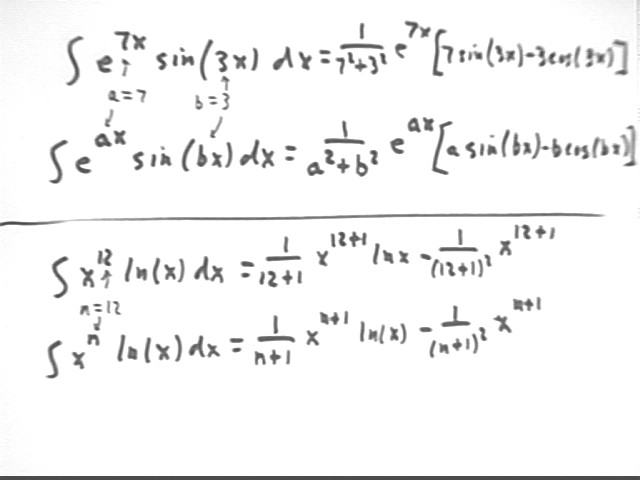
integral ( e^(7x) * sin ( 3x ) dx)
The first figure below shows how this integral matches the form given in the table, with a = 7 and b = 3. The evaluation of the integral using this formula is straightforward.
integral ( x^12 ln(x) dx )
The lower half of the figure below shows how this integral matches the form given in the table, with n = 12. The evaluation of the integral using this formula is again straightforward.
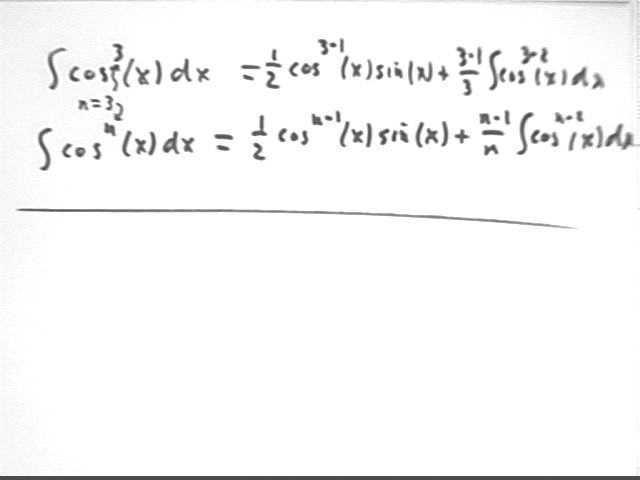
integral ( cos^3(x) dx ).
The figure below shows how this integral matches the form in the table, with n = 3.
Note the link to the Temple University site. This site comes highly recommended by one of our students. Try it and let me know how you like it.
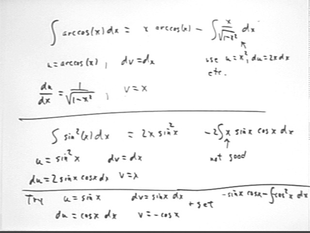
The figure below illustrates first how to integrate arccos(x) dx using the breakdown u = arccos(x), dv = dx.
We get du = 1 / sqrt(1-x^2) dx and v = x.
We integrate the resulting x / sqrt(1-x^2) using another substitution, this time u = 1 - x^2 so that the x dx in the integral becomes 1/2 du and the integrand simply 1 / sqrt(u).
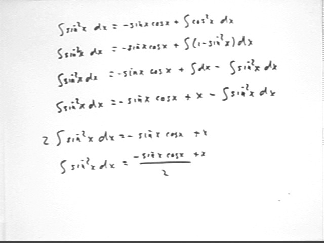
The second figure demonstrates the integral of sin^2(x).
We first try u = sin^2(x) and dv = dx. However that leads to the integral of x sin(x) cos(x), which doesn't look promising.
We next try u = sin(x), dv = sin(x) dx. We end up with an integral of cos^2(x), which at first doesn't seem to be an improvement over the original integral of sin^2(x) dx.
However the relationship between sin^2(x) and cos^2(x) gives us an opportunity to make some real progress, as in the next figure.
Using the fact that cos^2(x) = 1 - sin^2(x) we obtain the equations in the second and third steps below.
In the fourth step we use the fact that integral ( dx ) is just x.
In the fifth step we add integral (sin^2(x) dx) to both sides, obtaining an equation which we easily solve for integral (sin^2(x) dx ).
Our solution is integral (sin^2(x) dx ) = -[ sin(x) cos(x) + x ] / 2.