Calculus II Class 01/31
Calculus I Quiz 0131
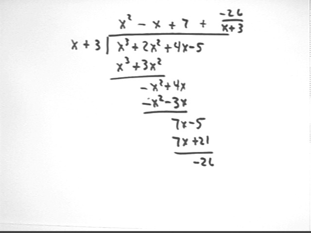
Divide x^3 + 2x^3 + 4x - 5 by x + 3 using long division. You'll end up with a polynomial and a fraction. Integrate the result.
The long division is illustrated below. At every step we divide the leading term of the divisor into the leading term of the dividend.
The thing to be most careful of is the step where we subtract expressions. For example subtracting -x^2 - 3 x from -x^2 + 4 x leaves us 4x - (-3x) = 7 x, not 4x - 3x = x.
When the degree of the divisor is greater than the degree of the numerator we simply place the remainder over the divisor and add the resulting expression to the quotient.
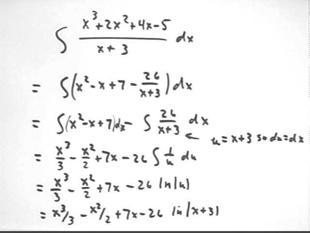
Using the result of the long division we easily integrate the quotient, as shown below.
The term 26 / (x+3) is integrated using u = x + 3 so that du = dx.
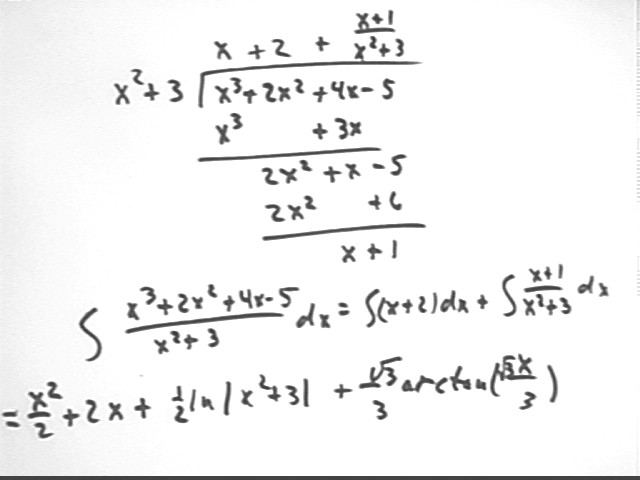
A similar expression but with x^2 + 3 in the denominator leads to the quotient expressed below.
Integrating the resulting expression we easily integrate the polynomial x + 2. However it takes a bit more work to integrate (x + 1) / (x^2 + 3).
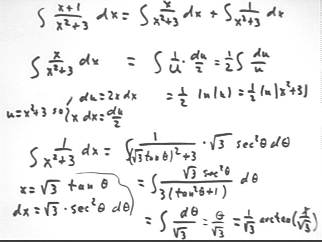
We write integral( (x + 1) / (x^2 + 3) ) as integral (x / (x^2 + 3) + integral (1 / (x^2 + 3) ).
integral (x / (x^2 + 3) ) is easily performed with the substitution u = x^2 + 3 so that du = 2 x dx and x dx = du/2, so that the integral becomes integral( 1/u * du/2) with result 1/2 ln(u) = 1/2 ln(x^2 + 3 ). This process is illustrated in the second figure below.
The integral of 1 / (x^2 + 3) is done using a trigonometric substitution, as shown in the next two figures. The result of this integral is sqrt( 3 ) / 3 arctan( sqrt(3) x / 3).
The figure below illustrates the integration of x / (x^2 + 3) and indicates the substitution x = sqrt(3) tan(theta) and the result 1/sqrt(30 * arctan(x / sqrt(3) for the integral of 1 / (x^2 + 3). The details of the second integration are illustrated in the next figure.
The first step below repeats the breakdown into two integrals of integral( (x+1) / (x^2 + 3) dx).
The second step repeats the integration of x / (x^2 + 3) using the substitution u = x^2 + 3.
The bottom half of the page illustrates the integration of 1 / (x^2 + 3) using the trigonometric substitution.
The substitution x = sqrt(3) * tan(theta) gives us dx = sqrt(3) * sec^2(theta).
The resulting integral { sqrt(3) sec^2(theta) / [ 3 ( tan^2(theta) + 1) ] d`that} simplifies, using the fact that tan^2(theta) + 1 = sec^2(theta), to just integral ( d`theta / sqrt(3) ), with the results indicated in the last step.
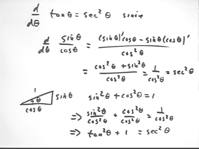
The derivative of tan(theta) and the origin of the identity tan^2(theta) + 1 = sec^2(theta) are illustrated below. Be sure to review thoroughly the section on trigonometry in the review chapter of your text.
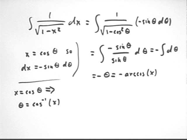
We illustrate now the integration of the expression 1 / sqrt( 1 - x^2)
Using x = cos(theta) we obtain dx = - sin(theta) d`theta.
The integrand becomes -sin(theta) / sqrt(1 - cos^2(theta) ) which by the Pythagorean identity becomes -sin(theta) / sqrt( sin^2(theta) ) = -sin(theta) / sin(theta) = -1.
The integral is therefore -theta, which we translate back into the original variable x to obtain our result -arccos(x).
Divide the region under the curve y = e^(-x^2) between x = 0 and x = 2 into four equal subintervals and find the trapezoidal approximation to the area under the curve.
The interval from x = 0 to x = 2 is divided into four subintervals using the partition { 0, .5, 1, 1.5, 2 }. The corresponding values of e^(-x^2) are given in the table below.
| x | e^(-x^2) | trap. area |
| 0 | 1 | |
| 0.5 | 0.778801 | 0.4447 |
| 1 | 0.367879 | 0.28667 |
| 1.5 | 0.105399 | 0.11832 |
| 2 | 0.018316 | 0.030929 |
| total area -> | 0.880619 |
The area of each trapezoid is the product of average altitude and width, with average altitude being the average of the two altitudes of the trapezoid.
The area of the first trapezoid, for example, is ave altitude * width = ( 1 + .7788 ) / 2 * .5 = .4447.
The areas of the remaining trapezoids are as indicated in the table, with the total .8806 indicated.
Find the midpoint approximation to the area under the curve in the preceding. You do this by using the midpoint 'height' of the actual function on each region instead of the straight-line approximation used in the preceding.
The figure below indicates the same partition as used for the trapezoidal approximation. However instead of approximating the areas by trapezoids we approximate by rectangles, with the altitude of each rectangle equal to the midpoint altitude not of a trapezoid but of the actual curve.
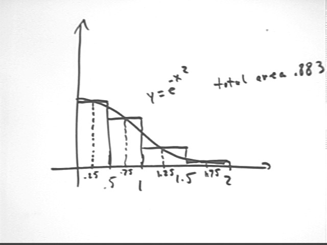
The table below indicates midpoint x values .25, .75, 1.25 and 1.75. The corresponding function values are indicated.
The area of each rectangle is midpoint altitude * width.
For example the area of the first rectangle is midpoint altitude * width = .9394 * .5 = .4697.
The total of all areas is .8828, as indicated.
| midpt x | fn value at midpt x | area of rectangle |
| 0.25 | 0.939413 | 0.469707 |
| 0.75 | 0.569783 | 0.284891 |
| 1.25 | 0.209611 | 0.104806 |
| 1.75 | 0.046771 | 0.023385 |
| Total area -> | 0.882789 |
The downward concavity of the curve on the first interval results in a trapezoidal approximation which is lower than the midpoint approximation. This is because the midpoint of the top segment of the trapezoid is lower than the midpoint of the actual curve, so that the average altitude of the trapezoid is less than the midpoint altitude of the function.
The upward concavity of the graph for the last two intervals entails a trapezoidal segment lying at its midpoint above the curve, which results for each of these intervals in a trapezoidal approximation which is greater than the midpoint approximation.
The concavity changes at x = sqrt(2)/2, within the second interval. The trapezoidal approximation is very slightly greater than the midpoint approximation, indicating that the trapezoidal segment lies at it midpoint slightly above the curve. The trapezoidal segment on this interval will therefore intersect the curve slightly past its midpoint.