Calculus II Class 02/24

It rained again.  After the rain seemed to be over I dumped one bucket into the other and got about a 5.5-inch depth.  Then it rained some more and I ended up with .5 inch of water in the bottom of the empty bucket.

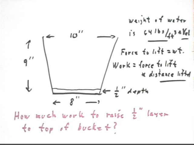
How much work would it take to raise that water to the level of the top of the bucket?

The figure below depicts the bucket and the information needed to calculate the weight of the water once we know its volume, then the work corresponding to the distance it is lifted.

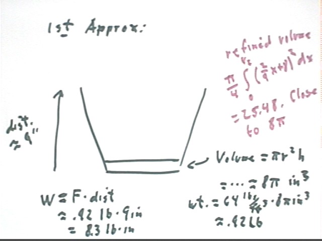
Simplest approximate answer:  You've got to raise that water 9 inches (or 8.5 inches or 8.75 inches, depending on how you think about it).  The weight of the water is found by first finding volume then multiplying by density.  So we have

• volume is approx. volume of cylinder diameter 8 in altitude .5 inch, so volume is 

V = area of base * altitude = pi * (4 in)^2 * .5 in = 8 pi in^3.

• weight = density * volume = 64 lbs / ft^3 * (8 pi in^3) = 512 pi in^3 / ft^3 lbs = 512 pi (in/ft)^3 lbs = 512 pi ( 1 in / (12 in) )^3 lbs = 512 pi (1/12)^3 lbs = .92 lbs. approx.

Now we easily calcuate work = force * distance = .92 lbs * 9 inches = 8.3 lb in.

We now note that our volume estimate is a bit low, being based on the cross-sectional area of the bottom of the container.  The cross-sectional area increases as we move upward.

• Recalling the analysis from an earlier class we see that the cross-sectional area at altitude x is pi/4 ( 2x/9 + 8)^2.  This cross-sectional area is integrated from the bottom of the container to the .5 inch height to obtain the more accurate result 25.48 in^3, close to but still noticeably different from our estimate 8 pi = 25.13.

We also note that we assumed that the entire quantity of water was raised 9 inches, when some of the water is only 8.5 inches below the top of the container.   We will next give a more accurate answer to a more specific question.

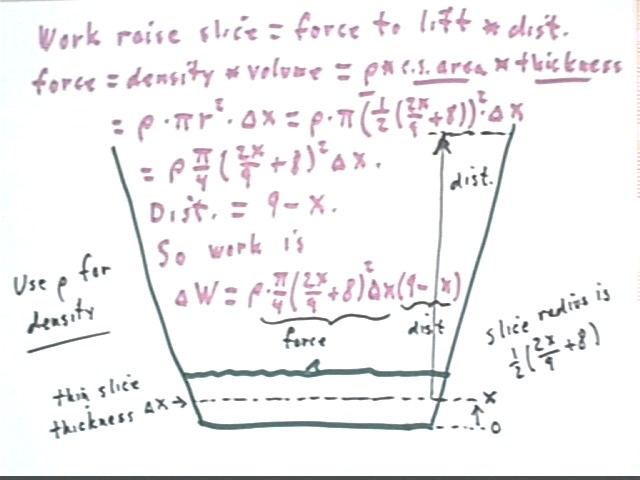
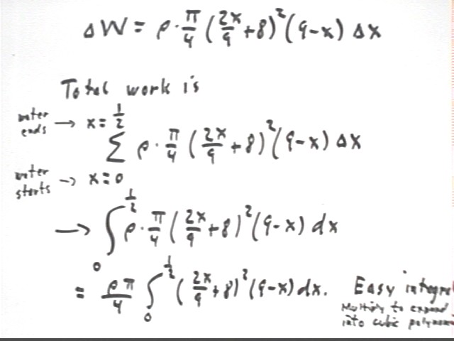
Now we refine the calculation.  What is the work required to raise to the rim of the bucket a 'slice' having thickness `dx with the slice at altitude x with respect to the bottom of the bucket?  Use rho for the density of the water.

From previous analysis we know that the radius of the slice is 1/2 (2 x / 9 + 8)^2.

It follows that the area of the slice is pi r^2 = pi [ 1/2 ( 2x/9 + 8)^2 ] = pi/4 (2x/9+8)^2 and its volume is 

• `dV = pi/4 (2x/9+8)^2 * `dx.

Its weight will be 

• wt = rho * `dV = rho * pi/4 (2x/9+8)^2 * `dx.

This weight is the force required to lift the water.

The distance is the vertical distance from position x to position 9 inches, so 

• dist = 9 - x.

The work contribution is therefore

• `dW =  rho * pi/4 (2x/9+8)^2 * `dx * (9-x).

Summing and taking the limit we get the integral indicated in the figure, which can be expanded into a polynomial and easily integrated.  The integral is 8.257431907, pretty close to the 8.3 obtained above.

Suppose you have an income stream of $1000 / month, flowing continuously into a bank account that earns 5% interest, compounded continuously.  Starting today you're gonna leave the money in the account for 10 years.

Recall that an initial amount P0 compounding continuously for T years at rate r grows to P0 * e^(r T).

How much will the money that flows into the account during the 27th month be worth at the end of the 10 years?

We know that $1000 flows into the account during that month.

We also know that the money will grow until the end of the 10th year, or the end of the 120th month.  So it seems that it has (120 - 27) months = 93 months = 93/12 years to grow.  But the money flows in during the interval from t = 27 months to t = 28 months, so the average t is about 27.5 months and the money only has an average of about 92.5 months to grow.

The result of $1000 growing for T = 92.5 months = 92.5 / 12 years is 

• final amount = $1000 * e^(.05 * 92.5 / 12).

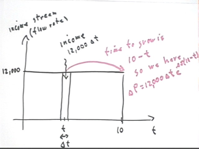
So to how much does the money grow which flows in during time interval `dt, near time t?

We need to ask how much money flows into the account during the time and how long it still has to grow.

• We'll assume that t is in years, so the rate at which money flows into the account will be $12,000 per year.
• Amount flowing in during time interval `dt (number of years in the time interval) is 12,000 * `dt.
• Time remaining for that money to grow is the time T from t to 10, or T = 10 - t.

So the money grows to final amount `dP = P0 * e^(r T) =   12,000 * `dt * e^(.05 ( 10 - t)).

The figure below depicts income stream (the 'flow rate' of the income) vs. clock time.

• For an interval of width `dt near clock time t the area beneath the graph represents the product of the income stream and the time interval `dt, i.e., the product of 'income flow rate' and time interval.  The result is the income we obtain during the time interval `dt.
• For income stream = $12,000 / year this amount is 12,000 * `dt.
• This income has 10 - t years to grow, so it grows to amount `dP = 12,000 * `dt * e^(.05(10-t)).

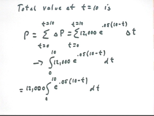
The total value of the entire 10-year income stream at the end of the 10 years is approximated by the sum of the contributions `dP = 12,000 * `dt * e^(.05(10-t)) from a set of time intervals spanning the 10-year period.  As the interval length `dt approaches zero the sum approaches as its limit the indicated integral.

This integral is easily evaluated using the substitution u = .05 ( 10 - t).

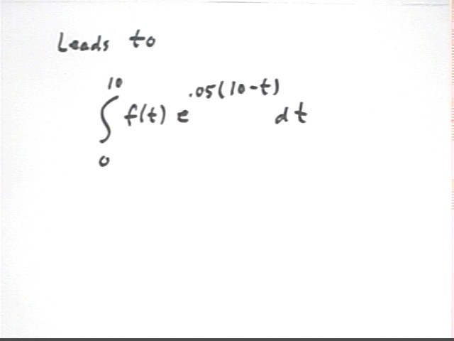
If the income stream if given by an 'income flow rate' function y = f(t), rather than a constant function, then the procedure followed previously need be only slightly modified, as depicted in the figure below.

• The income for a time interval `dt near time t will now be f(t) * `dt.
• This income, as in the previous case, has 10 - t years to grow.
• This income therefore grows to value `dP = f(t) `dt * e^(.05 ( 10 - t) ).

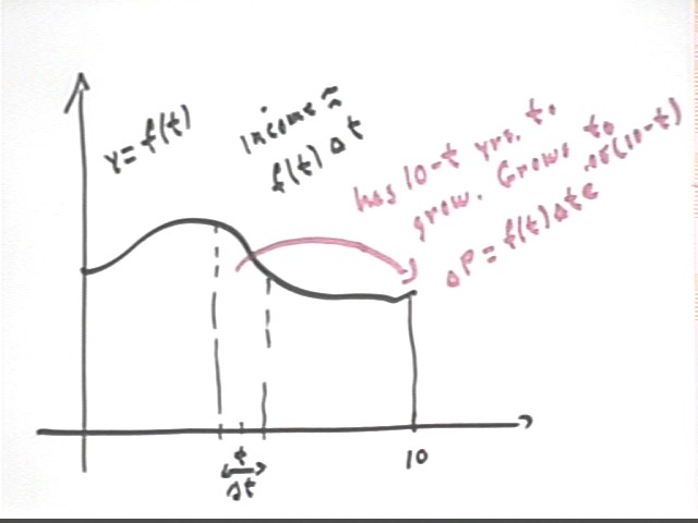
Summing these contributions in the same manner as before leads to the integral depicted in the figure below.

• In the previous example f(t) was the constant function $12000 / yr.  Replacing f(t) by 12,000 we get the integral of the previous example, in which the 12,000 was constant and could be factored out of the integral.
• If f(t) is not constant then it cannot be factored out of the integral.  Since f(t) must remain in the integral we will no longer have a simple antiderivative and will likely have to attempt integration by parts.  It is very possible that our expression cannot be integrated.

If f(t) is a polynomial we will be able to find the integral using integration by parts.

If f(t) is an exponential function of t we will be able to combine the exponential functions into a single exponential function and easily get an antiderivative by substitution.

For other functions f(t) we might or might not be able to accomplish the integration.   Even if we can't numerical approximations can give us good results.