Calculus II Class 03/10

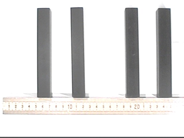
The figure below depicts a side view four bars balanced on a meter stick.  We wish to find the location of the balancing point.  If the mass of the meter stick is negligible and if the mass of each bar is 300 grams, we calculate the 'torque' of each bar about the left-hand end by calculating the moment of each, which 300 grams * moment arm, and summing all 'torques'.  (Note that these aren't really torques because torque is force * moment arm and 300 grams is not a force but rather a mass.  Gravity exerts its force on the mass and it is this force that results in torque.  However that's a fine point that we can leave to physics students.  Here we'll treat the mass like a force.) 

• The locations of the masses are approximately 6 cm, 11.5 cm, 19.5 cm and 24.5 cm from the left end.  Their torques (multiply each mass by the distance and understanding that the units are gram * cm) are therefore approximately 1800, 3450, 5850 and 7350.
• The total torque is the sum 1800 + 3450 + 5850 + 7350 = 18450.
• This torque tends to rotate the system in the clockwise direction.

If the system is balanced at a point xMean then the total 1200 grams must be supported at this point, and the torque exerted by the balancing point must be 1200 grams * xMean in the counterclockwise direction.  Since this torque must exactly balance the clockwise torque exerted by gravity our two torques 18450 gram cm and 1200 grams * xMean must be equal in magnitude.  We therefore have

• 1200 grams * xMean = 18450 gram cm

which we easily solve to get

• xMean = 18450 gram cm / (1200 grams) = 15.4 cm, approx.

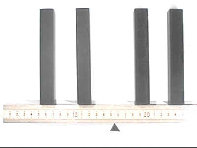
The figure below shows the system balancing at its center of mass.

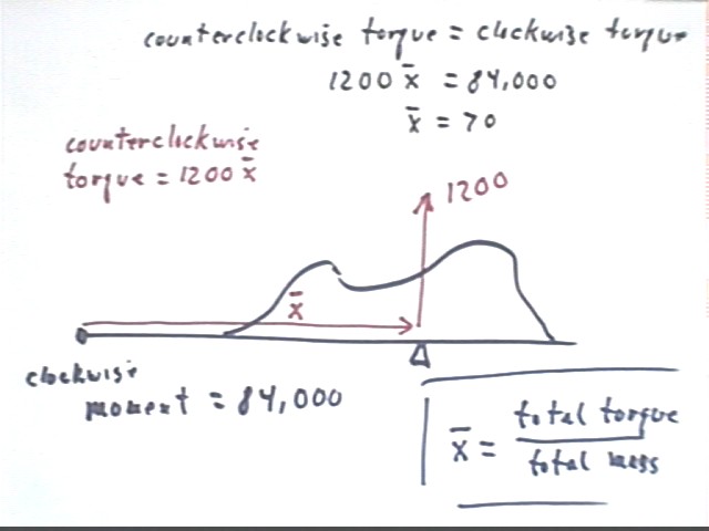
Another system, with a continuous mass distribution, is analyzed by summing the masses and the torques about the x = 0 point to have total mass 1200 grams and total clockwise torque (also called clockwise moment) 84,000 gram cm.

If the balancing point of the system is at xMean, represented by the x with the bar over it, then the support must exert a enough upward force to support the 1200 grams at distance xMean from the pivot at x = 0.  The counterclockwise moment, or torque, will be 1200 * xMean. 

• Since the system is stationary the counterclockwise and clockwise torques must be equal so that 1200 xMean = 84,000 and xMean = 70.

Thus the system balances at point xMean = 70.

We generalize this procedure to probability distributions.  Instead of mass we will be using area and we will be using Riemann Sums which approach the integrals we will evaluate.

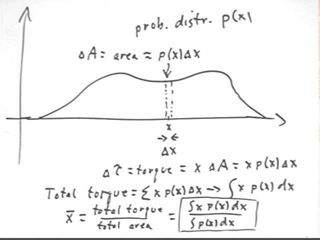
The figure below represents a probability distribution p(x).  Instead of one of the metal bars in the initial example we use a thin slice of the distribution having width `dx and located near position x. 

• This slice will have height p(x) and width `dx so its area is `dA = p(x) `dx.
• The torque of the slice will be the product of its area and its moment-arm.   Calculating the moment about x = 0 we obtain torque = `dTau = moment arm * area = x * `dA, which leads us to

torque increment = `dTau = x * `dA = x * p(x) `dx.

The mean xMean will as before have the property that xMean = total torque / total mass, or in this case where mass is represented by area, xMean = total torque / total area.

Total torque is the sum of all the `dTau contributions, which as `dx shrinks toward zero approaches the integral of x p(x) with respect to x.

Total area is the sum of all the `dA contributions, which as `dx shrinks toward zero approaches the integral of p(x) with respect to x.

• We therefore obtain xMean = total torque / total area = integral( x p(x) dx) / integral (p(x) dx).

If p(x) is a probability distribution then the total area beneath its graph is 1 and the denominator is therefore 1, so we have

• For probability distribution p(x):  xMean = integral ( p(x) dx).

The integral in every case extends from -infinity to infinity.  Note that many probability distributions are defined only over a finite interval or a half-infinite interval (e.g., for x > 0) and are therefore considered zero elsewhere.

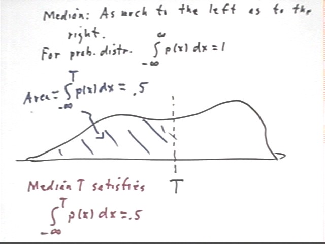
The median of a distribution is the 'middle' of the distribution in the sense that the median is that location in the distribution for which the probability to the left is .5 and the probability to the right is .5.

If we let T stand for the median then the condition for T is that probability( x < T ) = probability (x > T) = .5.

If probability (x < T) = .5 it follows that probability(x > T) = .5.  Since probability(x < .5) = integral (p(x) dx from x = -infinity to T) our definition of the median is

• The median is the value of t for which integral (p(x) dx from x = -infinity to T) = .5.

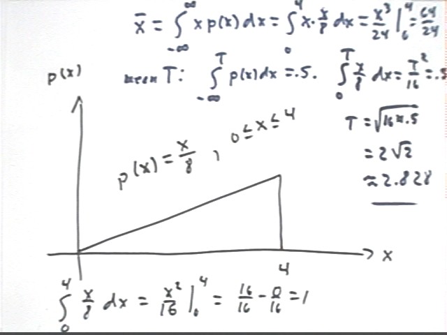
If p(x) = x/8, 0 < x < 4, with p(x) = 0 elsewhere then

• Is p(x) a probability distribution?

A probability distribution must be nonnegative and its integral from -infinity to infinity must be 1.

• For 0 < x < 4 we see that 0/8 < x/8 < 4/8 or 0 < p(x) < .5 so p(x) is nonnegative.

p(x) = 0 for x < 0 and for x > 0 so its integral from -infinity to infinity is just int(x/8), x, 0, 4).  We show that this integral is 1:

• Antiderivative is x^2 / 16; change in antiderivative from x = 0 to x = 4 is 4^2/16 - 0^2 / 16 = 1 - 0 = 1.  So we have a probability distribution.

• What is the median?

Median is T such that int(x/8,-infinity, T) = .5.

• The integral becomes int(x/8, 0, T), which is T^2 / 16.
• The integral is equal to .5 when T^2 / 16 = .5, or T = sqrt(8) = 2 sqrt(2), approx. 2.828.

• What is the mean?

Mean is

• xMean = int(x p(x), x, -infinity, infinity) = int(x * x/8, 0, 4).
• This integral is easily evaluated, as shown below, to obtain xMean = 64/24 = 8/3 = 2.67 approx..

We therefore have

• mean = 2.67 approx.
• median = 2.828.

Note that the mean and median are not generally the same, though for some distributions they do coincide.

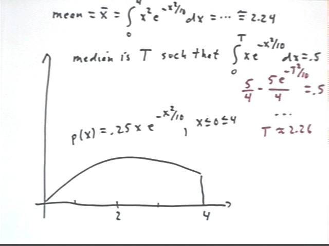
Recall the probability distribution function for a player whose density function is e^-(x^2/10).  We saw before that this density function leads to the probability function p(x) = .25 x e^-(x^2/10).  (The .25 is the constant needed to make the integral of p(x), from -inf to inf, equal to 1, so we know that this is a probability distribution.)

Find the mean and median for this distribution.

• Mean = int(x p(x), x, -infinity, infinity) = int(x * .25 x e^(-x^2/10), x, 0, 4)

Introduction to Sequences and Series

Consider someone who wants to travel 8 feet but isn't sure how to go about it.   This person first travels half the distance, 4 feet, then travels have the remaining distance or 2 feet, then again half the remaining distance or 1 foot.  The person continues in this manner.

• It should be clear that the total distance is 4 + 2 + 1 + 1/2 + 1/4 + 1/8 + ... , where ... indicates that the sum continues forever.
• It should also be clear that the total distance will be 8 feet so that the sum 4 + 2 + 1 + 1/2 + 1/4 + 1/8 + ... = 8.
• The numbers 4, 2, 1, 1/2, etc. are of the form 8/2, 8/4, 8/8, 8/16, ... .  These numbers can be represented as 8/2^1, 8/2^2, 8/2^3, 8/2^4, ...  So the sum can be expressed as sum(8 / 2^n, n from 1 to infinity).

The figure at the bottom of the page indicates how the sum can be represented by the total area of a series of rectangles along the x axis.

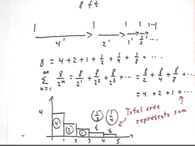
Now observe the following:

• The upper right-hand corners of the rectangles representing the sum 4 + 2 + 1 + 1/2 + ... have coordinates (1, 4), (2, 2) , (3, 1), (4, 1/2) etc.  The coordinate of the nth upper-right-hand corner point is therefore 8 / 2^n.
• It follows that the rectangles all lie beneath the graph of the function y = 8 / 2^x.

• The upper left-hand corners of the same rectangles are at (0, 4), (1, 2), (2, 1), (3, 1/2), etc.  The coordinate of the nth upper-left-hand corner point is therefore 8 / 2^(n+1).
• Thus the graph of y = 8 / 2^(x+1) lies entirely within the rectangles.

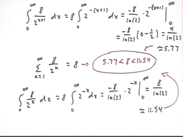
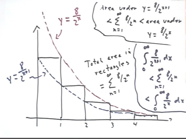
We conclude that the total area of all the rectangles is less than the area under the y = 8 / 2^x curve for x > 0, and the total area of all the rectangles is greater than the area under the y = 8 / 2^(x+1) curve for x > 0.

• Another way of saying this is

integral(8 / 2^(x+1) dx for x from 0 to infinity) < sum(8 / 2^n for n from 1 to infinity) < integral(8 / 2^x dx for x from 0 to infinity.

This inequality is written in conventional notation in the figure below.

If we evaluate the integrals and the sum we verify the inequality

• The sum 4 + 2 + 1 + 1/2 + ... was seen earlier to be 8.
• The integrals have values approximately equal to 5.77 and 11.54.  Since 5.77 < 8 < 11.54 the inequality is verified.