Calculus II Class 03/26
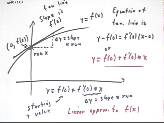
The tangent line to the graph of y = f(x) at x = 0 passes through the point (0, f(0)).
The slope of the tangent line at a point is equal to the derivative of the function at the point. So the slope of the tangent line is
The equation of the tangent line, using slope-intercept form, is therefore
which we easily rearrange to give us
This form is also easily obtained using the 'slope triangle', which shows that `dy = slope * run = f ' (0) * x. The y value at x will therefore be the sum of the original y value and the change `dy in y, i.e., y = f(0) + f ' (0) * x.
This approximation is called the First Degree Taylor Polynomial, denoted P1(x):
This polynomial matches the value and the slope of the function at x = 0.
This linear approximation of a continuously differentiable function works fine near the x = 0 point, but unless the function is linear the accuracy of the approximation tends to decrease as we move away from x = 0.
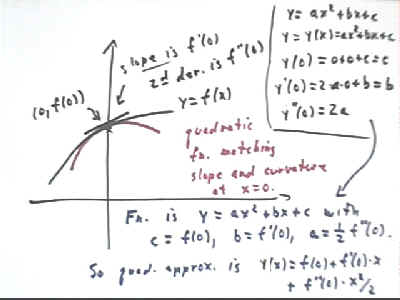
We can match the curvature of the function near x = 0 by doing a quadratic approximation whose value, first and second derivative match those of f(x).
If we let y = y(x) = a x^2 + b x = c be our approximation then we find that y(0) = c, y ' (0) = b and y '' (0) = 2a. If these values match f(0), f ' (0) and f '' (0) then we have
In this case our approximating function is y(x) = 1/2 f ''(0) x^2 + f ' (0) x + f(0), or reversing the order to mimic the order of a power series, and also denoting this function by P2(x) we have
We call this our Second Degree Taylor Polynomial.
A quadratic function has a constant second derivative. It cannot, for example, change its concavity. Some functions do change concavity, and many have changing second derivatives.
Since y = x^3 changes concavity it can help us more accurately model other functions that also change concavity.
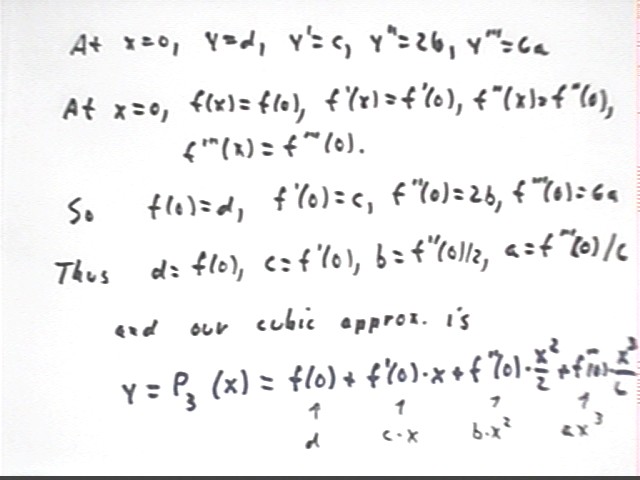
We can use a cubic polynomial to match the value and first three derivative of f(x) at x = 0, as incidated in the figure below.
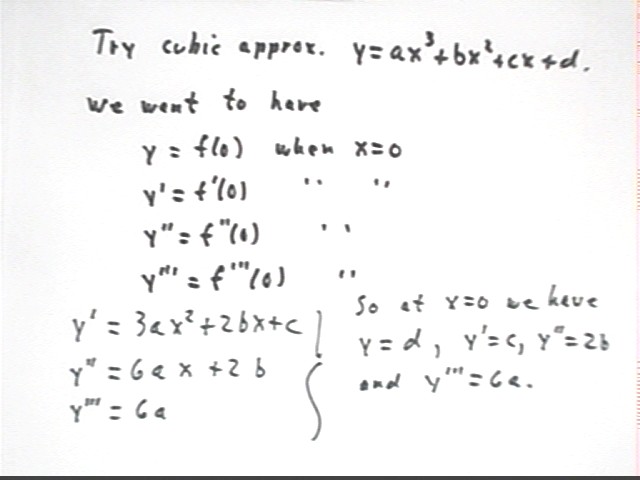
If these values match f, f ' , f '' and f ''' at x = 0 then as shown in the figure below we have
Our cubic polynomial is therefore y = f ''' (0) / 6 * x^3 + f '' (0) / 2 * x^2 + f ' (0) * x + f (0), or using P3(x) as the label for this function and again reversing order:
The Taylor polynomials are therefore
P1(x) = f(0) + f ' (0) * x
P2(x) = f(0) + f ' (0) * x + f '' (0) * x^2 / (2 * 1)
P3(x) = f(0) + f ' (0) * x + f '' (0) * x^2 / (2 * 1) + f '''(0) * x^3 / (3 * 2 * 1)
P4(x) = f(0) + f ' (0) * x + f '' (0) * x^2 / (2 * 1) + f '''(0) * x^3 / (3 * 2 * 1) + f ''''(0) * x^4 / (4 * 3 * 2 * 1)
P4(x) = f(0) + f ' (0) * x + f '' (0) * x^2 / 2! + f '''(0) * x^3 / 3! + f ''''(0) * x^4 / 4!
2d derivative of a x^2 is 2 * 1 * a, which is where that 2! comes from
3d derivative of a x^3 is 3 * 2 * 1 * a, which is where that 3! comes from
4th derivative of a x^4 is 4 * 3 * 2 * 1 * a, which is where that 4! comes from
nth derivative of a x^n: derivative sequence is
The final result is n ( n-1) (n-2) * ... * 3 * 2 * 1, or n !
The nth degree approximation is therefore
Pn(x) = f(0) + f ' (0) * x + f '' (0) * x^2 / 2! + f '''(0) * x^3 / 3! + f ''''(0) * x^4 / 4! + ... + f[n] * x^n / n!,
where f[n] indicates the nth derivative of f with respect to x.
Find the 4th-degree Taylor polynomial approximation to y = f(x) = sin(x) near x = 0.
P4(x) = f(0) + f ' (0) * x + f '' (0) * x^2 / 2! + f '''(0) * x^3 / 3! + f ''''(0) * x^4 / 4!
All we need to find is f(0), f ' (0), f '' (0), f ''' (0) and f '''' (0).
Thus we have
P4(x)
= 0 + 1 * x + 0 * x^2 / 2! + (-1) * x^3 / 3! + 0 * x^4 / 4!
= x - x^3 / 3!
= x - x^3 / 6.
How close is P4(x) to sin(x) when x = .1?
P4(x) = x - x^3 / 6 so
P4(.1) = .1 - .1^3 / 6 = .1 - .000166 = .0998333333...
sin(.1) = .09983342
The figure below illustrates y = sin(x) along with the third-degree Taylor approximation P3(x) = x - x^3 / 3!.
The third-degree polynomial approaches infinity as x moves through large negative numbers, and approaches -infinity as x moves through large positive numbers. So the polynomial must eventually deviate from the sine function.
A cubic polynomial can have at most two changes in direction (due to the fact that its derivative is quadratic it can have at most 2 critical points) and is for that reason limited to at most one period of the sine function.
The figure below illustrates y = sin(x) along with the fifth-degree Taylor approximation P5(x) = x - x^3 / 3! + x^5 / 5! and the previous third-degree polynomial.
The fifth-degree polynomial approaches -infinity as x moves through large negative numbers, and approaches infinity as x moves through large positive numbers. So the polynomial must eventually deviate from the sine function.
A degree-5 polynomial can have four changes in direction as opposed to two for the degree-3 approximation, allowing it to follow the sine function further than the P3(x).
The figure below illustrates y = sin(x) along with the 7th-degree Taylor approximation P7(x) = x - x^3 / 3! + x^5 / 5! + x^7 / 7! and the previous Taylor polynomial approximations.
The 7th-degree polynomial approaches infinity as x moves through large negative numbers, and approaches -infinity as x moves through large positive numbers. So the polynomial must eventually deviate from the sine function.
The figure below shows the degree-9 approximation P9(x) = x - x^3 / 3! + x^5 / 5! - x^7 / 7! + x^9 / 9!. This approximation works well at least for one period of the sine function on the interval -pi < x < pi.