Calculus II Class 04/14

Sketch a grid with short line segments, called 'slope segments', at every point on the grid we get when we intersect the lines x = 0, 1, 2, 3 with the lines y =  0, 1, 2, 3 (i.e., the points (0, 0), (0, 1), ... (0, 3), (1, 0), (1, 1), ..., (1, 3), (2, 0), etc.).    The slope of each segment should be y / 2, where y is the y coordinate of the point.

We get the figure below. 

• At each point where y = 0--i.e., on the x axis-- the slope is 0 and the segment is horizontal. 
• At each point where y = 1--i.e., on the horizontal line y/2 = 1/2, lying 1/2 unit above the x axis-- the slope is 1 and the segment is at a 45 deg angle to the horizontal.
• At each point where y = 2--i.e., on the horizontal line y = 2, lying 2 units above the x axis-- the slope is y/2 = 2/2 and the segment the 'rise' of the segment is double the 'run'.
• In the next figure we have indicated the lines y = -3, y = -2, ..., y = 3.  You should see that the slope segments along each line are constant and equal to y / 2.

Suppose that an air or water current has the direction indicated by the slope field.  Sketch a set of curves indicating the path of an object drifting in this current.  Start one path around the point (0, 1), another around (0, 1/4) and another to the left of both of the first two curves.

The figure below indicates approximate paths, constantly curving to adjust to the changing direction of the slope field.

Since slope can indicate the rate at which y changes with respect to x, our sketch represents the slope field for the differential equation

• dy/dx = 2 y.

The resulting curves indicate solutions of the equation.  The slope field allows us to graphically approximate the solutions to a differential equation, even if we cannot find the exact form of the function which solves it.

For the given equation we can find a solution without too much difficulty, as we saw in the preceding class.

• The general solution to this equation is found by rewriting the equation as dy / y = dx / 2, and integrating both sides. 
• The final result is the family of solutions  | y | = C e^(x/2), where C is an arbitrary constant greater than 0.
• This family of solutions 'fits' the slope field perfectly, giving us precise versions of the curves we have sketched.

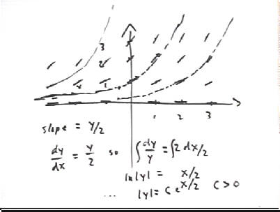
The figure below depicts this direction field with graphs of the solutions | y | = C e^(x/2) for C = 0, .5, 1, 1.5, 2, 2.5 and 3.  We see how these solutions fit the slope field, in the sense that an air or water current in the directions indicated by the slope field would cause an object at a point on one of these curves to 'float' in the direction of that curve.

For grid points in the first and fourth quadrants, from x = 0 to x = 3 and y = -3 to y = 3, sketch the slope field of the equation dy/dx = x - y (i.e., at every grid point the slope will be given by the value of x - y).  Sketch a few curves, some starting below the line y = x and some above.

Along the line y = -1 the y values 1, 2 and 3 result in slopes of 1 - (-1) = 2, 2 - (-1) = 3 and 3 - (-1) = 4.

Along the line y = 1 the x values 1, 2 and 3 result in slopes of 1 - 1 = 0, 2-1 = 1, 3-1 = 2.

Along the lines y = 0, y = 2 and y = 3 values are calculated similarly.  For y = 2 and y = 3 some of the values are negative, resulting in segments with negative slope.

Four approximate curves following this slope field are indicated below.

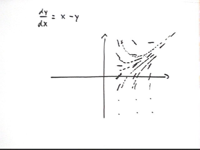
The figure below shows a more detailed and accurate slope field.

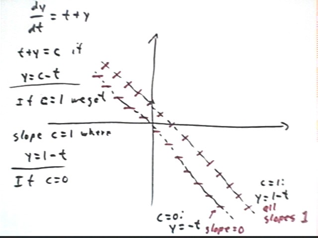
For the equation dy/dt = t + y the slope dy/dt is equal to a constant c whenever t + y = c.  Using slope-intercept form y = m t + b find the equations of the lines t + y = c for c = 1 and also for c = 0.  Sketch these lines on a y vs. t coordinate system

If c = 1 then t + y = 1 and we have y = -t + 1, a straight line with y intercept (0, 1) and slope -1.

If c = 0 then t + y = 0 and we have y = -t + 0, a straight line with y intercept (0, 0) and slope -1.

Along the c = 1 line the slope dy/dt should be 1.  Sketch a number of segments along this line, each segment having slope 1.  Then sketch on the c = 0 line a series of segments corresponding to c = 0.

The figure below depicts the two lines (the dotted lines) and the slope segments along each line.

Extend your figure to include the lines for c = -2, c = -1 and c = 2.

The lines are respectively y = -t - 2, y = -t - 1, y = -t + 2, depicted below.

Along each line is a series of slope segments whose slope is approximately equal to c.

An accurate picture of the slope field for the equation dy/dt = t + y is depicted below.  This slope field was not constructed using the dy/dt = c lines of the preceding figure, but by simply calculating the slope at each grid point.  You should see that the two methods produce the same slope field, but not using exactly the same points.

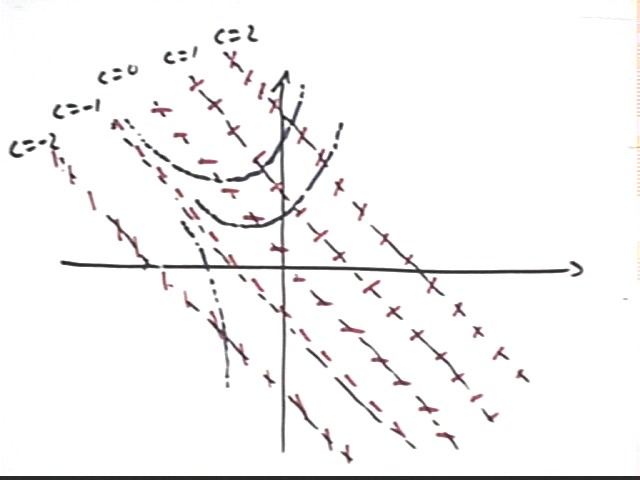
For the equation dy/dt = x^2 - y, sketch the curves for which dy/dt = c for c = -1, c = 0 and c = 1.  Along each curve sketch slope segments with appropriate slope.

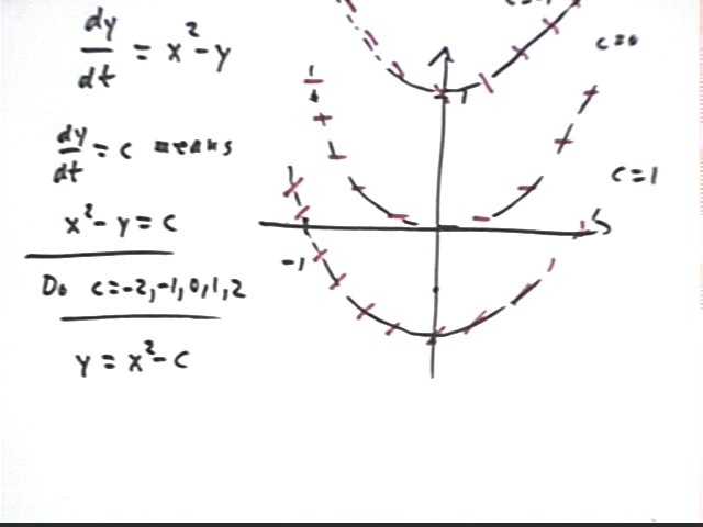
The same slope field plotted at grid points.  The curves y = x^2 + c for x = -4, -2, 0, 2 and 4 are depicted.  Note how the slopes at the points where these curves intersect the direction field are uniform along every curve.

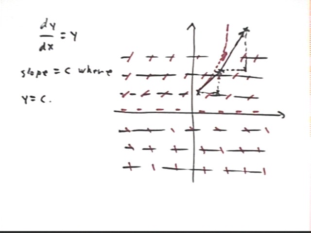
Look at the slope field for the curve dy/dx = y, shown below.  Find the point (.3, 1) and identify the slope at this point. 

We look at the figure and see that along the line y = 1 the slope is always 1.  Since (.3, 1) lies on the line y = 1, the slope at this point is 1. 

This must be the slope since the y coordinate is 1 and dy/dx = y. 

If we follow the direction of the slope at that point until x has changed by 1 unit then at what point will we arrive?

If we follow the slope at that point until x has changed by 1 unit, our y change will also be 1 unit, since the slope is 1.

The figure below shows vertical and horizontal lines intersecting at (.3, 1), and the line of slope 1 originating at that point.

More formally we know that rise / run = slope = 1 and that run = 1.  So our rise will be

• rise = slope * run = 1 * 1 = 1.

Starting from (.3, 1) and letting x and y both increase by 1 we will arrive at the point (1.3, 2).

If we had followed the slope field and not the straight line would y have increased by the same amount, by a greater amount or by a lesser amount than along the straight line?

You should see from the slope field that the actual path followed from the point (.3, 1) is not a straight line, since the slope should continue increasing as our y coordinate increases.  This will cause the actual path to curve away from the straight line, so that the straight-line approximation will be an underestimate.

The graph below shows the same slope line as before, and in addition the curving graph that actually follows the slope field.

Find the slope of the graph at (1.3, 2) and follow this slope while x again changes by 1.  At what point do you end up?

At (1.3, 2) the slope is 2.  If we follow this slope as x changes by another unit we arrive at the point (2.3, 4).

The figure below depicts this process in the context of the slope field.

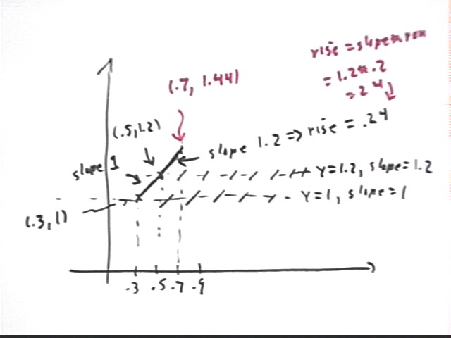
If we follos the same process, again starting at (.3, 1) but this time moving with an x increment of .2, we will obtain in successive steps estimates for x = .5, .7, .9, etc..

• Starting at ( .3, 1) we again find that the slope is 1.  Following this slope for a 'run' of .2 we arrive at x = .5.  The rise is `dy = slope * `dx = 1 * .2 = .2, so our new y coordinate is 1 + .2 = 1.2.
• Now starting at ( .5, 1.2) we find that the slope is y = 1.2.  Following this slope for a 'run' of .2 we arrive at x = .5.  The rise is `dy = slope * `dx = 1 * 1.2 = .24, so our new y coordinate is 1 + .24 = 1.44.
• If we were to continue we would find the slope at our new point (.3, 1.44) and follow it for an x increment of .2.
• Continuing in this manner we could be approximations for x = .9, 1.1, 1.3, ... as far as we wish.  Note however that since each approximation follows only the initial slope and doesn't adjust until the next point for the changing slope field, our approximations will be less and less accurate.

The figure below shows this process in the context of the slope field.

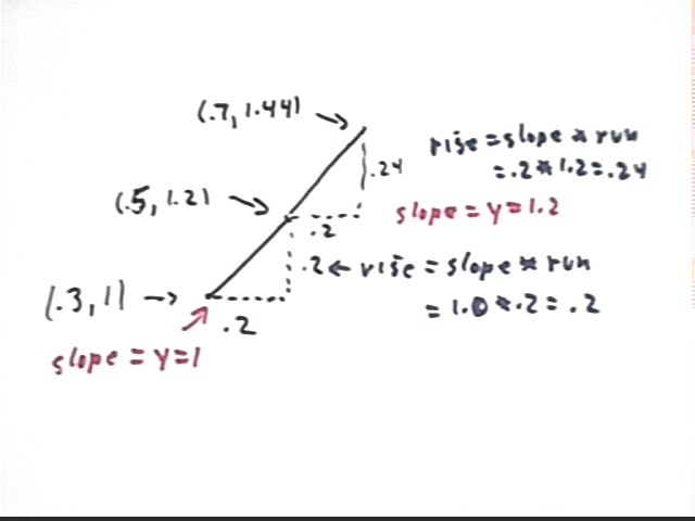
The next figure shows the details of each 'slope triangle' used in this calculation.

Slope fields for various differential equations are depicted below.  You should be able to construct these slope fields from the equations, by two methods:

• You should be able to sketch a slope field by simply calculating and sketching the slopes at grid points.
• You should also be able to sketch a slope field by finding the curves for which dy/dx = c for an arbitrary constant c, plotting the curves for a variety of c values, and sketching short segments of slope c along each curve.

dy/dx = y - x

dy/dx = x + y

dy/dx = -y/x

dy/dx = x^2 + y^2