Calculus II Class 04/28

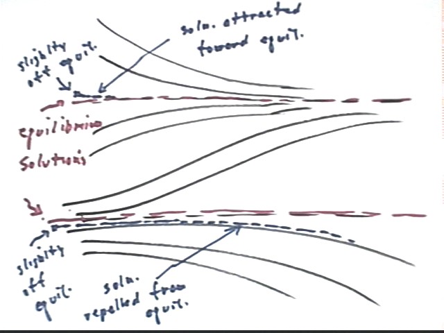
Consider a fertile pond with no fish in it.  No fish is an equilibrium state.  As long as you got no fish you're gonna continue to have no fish.

What do we have if we deviate slightly from this equilibrium state?

We have some fish.  If the deviation is slight then we have just a few fish. 

What happens next?

We get more fish, which in turn produce more fish, etc., etc.. 

However there are limits to how many fish we can have.  So eventually the population approaches the carrying capacity of the pond, which is another equilibrium state.

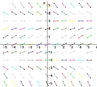
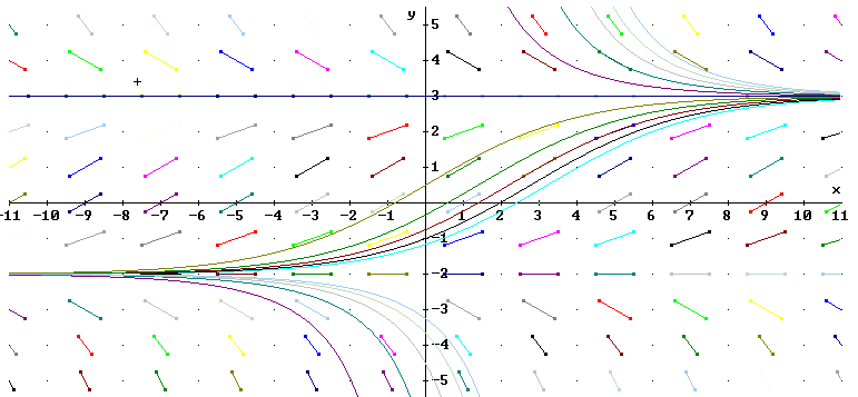
The figure below depicts the direction field for the equation

• dy/dt = -.1(y+2)(y-3)

Sketch a set of solution curves for this direction field.

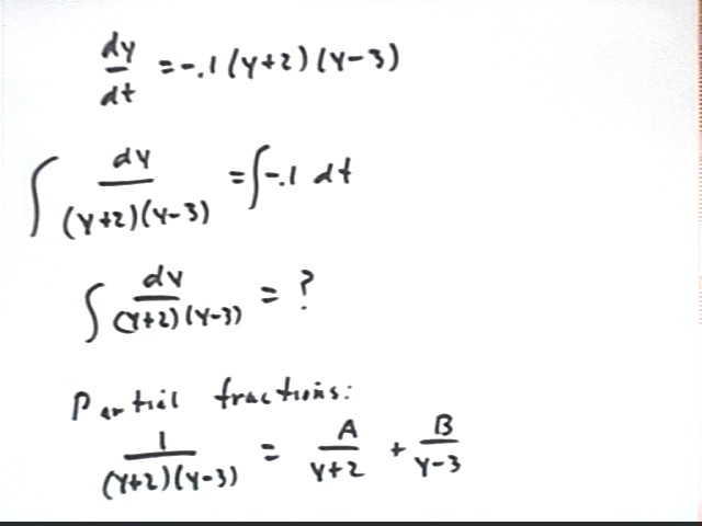
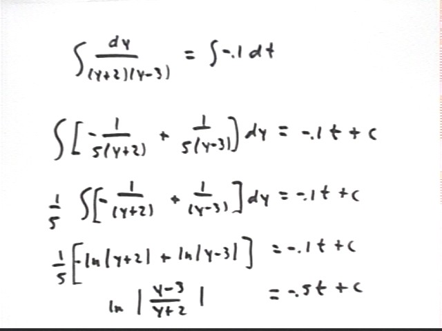
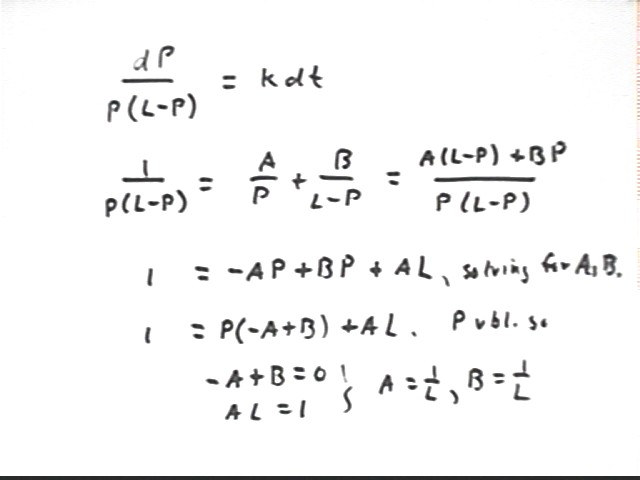
Solve the equation dy/dt = -.1(y+2)(y-3).

We easily separate variables to get

dy / [ (y+2)(y-3) ] = dt.

To integrate dy/ [ (y+2)(y-3) ] we use partial fractions:

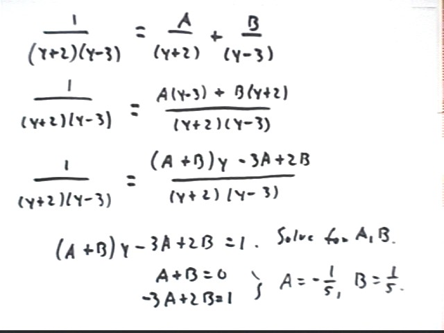
There exist A and B for which 1 / [ (y+2) (y-3) ] = A / (y+2) + B / (y - 3).

A / (y+2) + B / (y - 3) = [ A ( y - 3) + B ( y + 2) ]  / (y+2)(y-3).  Simplifying this expression we get

[ ( A + B ) y - 3 A + 2 B ] / (y+2)(y-3).

If

• [ ( A + B ) y - 3 A + 2 B ] / (y+2)(y-3) =  1 / (y+2)(y-3)

for all y then

• A + B = 0 and -3A + 2B = 1.

Solving for A and B we get

• A = -1/5, B = 1/5.

Thus

•  1 / (y+2)(y-3) = -1 / (5 (y+2) ) + 1 / 5(y - 3).

The solution (see details below; steps have been left out which should be familiar by this point) is

• y = (3 + 2 A e^-.5 t) / (1 - A e^-.5 t),

where A is any  nonzero constant.

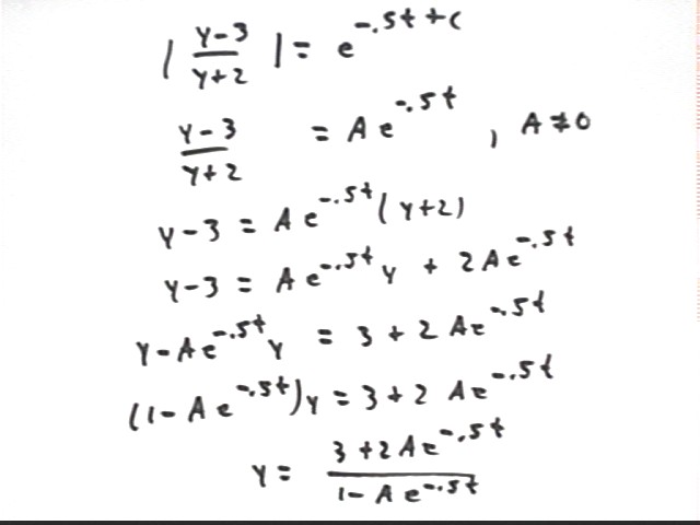
Plotting this family of solutions, for A = -10 to A = 10, along with the direction field we get the following:

.

Remember that the logistic equation, often applied to population growth in environments with limited carrying capacity, is

dP/dt = k P (L - P),

where L is the population at carrying capacity.

Note that this is just a modification of the exponential growth equation

dP/dt = k P,

multiplying by the factor L - P, which approaches zero at P approaches carrying capacity. 

For small P our equation dP/dt = k P (L - P) gives us a pretty constant growth rate, since for small populations L - P is pretty close to L.  So we start with something very much like exponential growth. 

To solve this equation, we first separate variables to get

dP / [ P ( L - P) ] = k dt.

We solve this equation using partial fractions, just like in the preceding example.  Details are shown below.

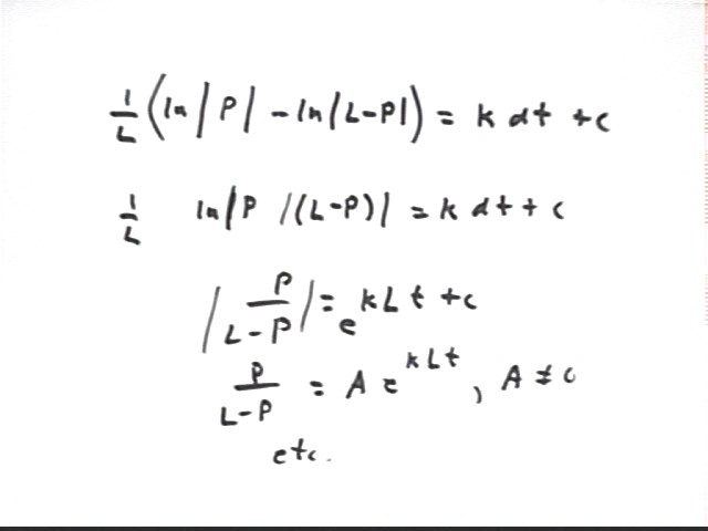
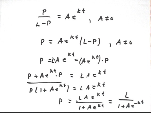
We end up with solution

P = L / (1 + A e^(-kt) ).

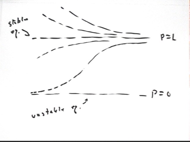
This function shows us that we have unstable equilibrium at 0, stable equilibrium at L.  That is, a small population moves away from the P = 0 equilibrium toward the stable equilibrium at P = L.

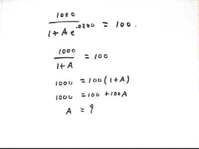
We can find the specific functions for a variety of different intial conditions.  For example if we know that the initial population is 100, carrying capacity is 1000 and the initial growth rate is 2% per unit of clock time then:

• The initial growth rate is k, so k = .02.
• At t = 0 the population is 100, so

P(0) = 1000 / (1 + A e^(.02 * 0) ) = 100.

We solve for A, obtaining  A = 9.

So P = L / (1 + A e^(kt) ) becomes

• P(t) = 1000 / (1 + 9 e^(-.02 t))

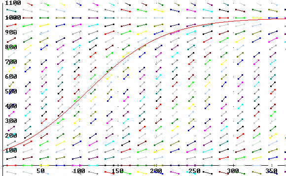
The direction field for this equation is shown below.  Note that the scale permits us to trace a solution curve from near the unstable equilibrium solution y = 0 to near the stable solution at y = 1000.

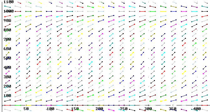
The solution obtained above for initial population y = 100 is shown with the direction field: