Calculus II Class 04/30

The velocity of water flowing from a small hole near the bottom of a uniform cylinder is

• vExit = sqrt(2 g y),

where g is the acceleration of gravity and y is the level of the water in the cylinder relative to the hole.

If the radius of the cylinder is R and the radius of the hole is r, then when water depth is y at what rate, in units of volume / unit of time, is water exiting the cylinder?

In time interval `dt the length of the stream that exits during this interval will be vExit * `dt = sqrt(2 g y) `dt.

In a short time interval `dt the corresponding short segment of the exiting stream will therefore be a cylinder with radius r and length sqrt(2 g y) `dt.  The volume of the cylinder is

• `dV = cross-sectional area * length = pi r^2 * sqrt(2 g y ) `dt

So the rate at which volume is exiting with respect to clock time is

• dV/dt = pi r^2 * sqrt(2 g y).

Looks like we have a differential equation, but with too many variables (V, t and y are all variable).

If we take V to be the volume of the water in the cylinder instead of the exiting volume then we can write

• dV/dt = - pi r^2 * sqrt(2 g y).

Are there any fixed relationships among V, y and t that would allow us to reduce the number of variables to 2?

There is no fixed relationship between V and t, since V changes at rates which change with t.  Similarly there is no fixed relationship between y and t.  However there is a simple fixed relationship between V and t.

The volume of water in the cylinder is cross-sectional area * height of the water column.  If we let V by just the volume above the hole then we have

• V = pi R^2 y.

Using the relationship V = pi R^2 y how can we express our differential equation dV/dt = -pi r^2 * sqrt(2 g y) ?

If V = pi R^2 y then since pi and R are constants

• dV/dt = pi R^2 dy/dt,

and our equation becomes

• pi R^2 dy/dt = -pi r^2 * sqrt(2 g y).

Solve the equation

• pi R^2 dy/dt = -pi r^2 * sqrt(2 g y)

for y as a function of t.

First note that pi R^2 and - pi r^2 sqrt(2g) are constant.  Dividing both sides by pi R^2 we get

• dy/dt = [ -r^2 / R^2 * sqrt(2 g) ] * sqrt(y).

Separating variables we have

• dy / sqrt(y) = [-(r/R)^2 * sqrt(2g)  ] dt.

Antiderivative of 1/ sqrt(y) is 2 sqrt(y) so we get

• 2 sqrt(y) = [-(r/R)^2 * sqrt(2g)  ] t + c

or

• sqrt(y) = [-(r/R)^2 * sqrt(g/2)  ] t + c

We need to solve for y so we square both sides to get

• y = [-(r/R)^2 * sqrt(g/2)  ]^2 t^2 - 2 [-(r/R)^2 * sqrt(g/2)  ] * t * c + c^2

or

• y = (r/R)^4 * g/2  t^2 + 2 c (r/R)^2 * sqrt(g/2) * t  + c^2.

This is a quadratic function of t.

Looks like a mess.  What do we get for a cylinder of radius 5 cm, hole radius .2 cm?

Substituting r = .2 cm, R = 5 cm and g = 980 cm/s^2, and suppressing units, we have

• y = (.2/5)^4 * 980/2  t^2 + 2 c (.2/5)^2 * sqrt(980/2) * t  + c^2

which simplifies to

• y = (.04)^4 * 490 t^2 + 2 c ( .04)^2 * 24.3 t + c^2.

or finally to

• y = .00125 t^2 + .0778 c t + c^2.

If the initial depth is 100 cm then what is the equation?

If y = 100 when t = 0 then we have

• 100 = .00125 * 0^2 + .0778 * c * 0 + c^2

which gives us c = 10.

Our equation is therefore

• y = .00125 t^2 + .778 t + 100.

The tube for which we found the quadratic depth vs. clock time model at the beginning of the course had radius 2 cm.  The hole radius was around 1.5 mm = .15 cm, initial depth was 90 cm.  What does our differential equation model give us for the y vs. t function?

r / R = .15 / 2 = .075, so we get

y = (r/R)^4 * g/2  t^2 + 2 c (r/R)^2 * sqrt(g/2) * t  + c^2

= (.075)^4 * 490 t^2 + 2 c ( .075)^2 * sqrt(490) * t + c^2

= .0155 t^2 + .125 c + c^2.

y = 90 when t = 0 so c = sqrt(90) = 8.4 approx. and our equation is

y = .0155 t^2 + .125 * 8.4 t + 90

= .0155 t^2 + 1.05 t + 90.

A model obtained for an actual cylinder, fitting data to a quadratic, is y = .0019 t^2 + .79 t + 90.  What hole diameter would correspond to this model?

The coefficient of t^2 = (r / R)^4 * 490 so we have

• .0019 = (r / R)^4 * 490, giving us

r / R = (.0019 / 490)^(1/4) = .044 approx.

If R = 2 cm as before then the hole diameter would be

• r = .044 R = .044 * 2 cm = .09 cm, approx..

This is reasonable, about 2/3 of the hole diameter assumed previously.  Note that the hole in the actual physical system had a bit of flexibility, so that the radius of the hole was probably greater when the water depth (and hence pressure) was greater.

Since the constant term is 90, our integration constant c is sqrt(90) = 8.4 as before.  Our coefficient of t should therefore be

• 2 c (r/R)^2 * sqrt(g/2) = 2 * 8.4 * (.044)^2 * sqrt(490) = .72.

This compares pretty well with the coefficient .79 of the model obtained from data.

Consider a fertile pond with no fish in it.  No fish is an equilibrium state.  As long as you got no fish you're gonna continue to have no fish.

What do we have if we deviate slightly from this equilibrium state?

We have some fish.  If the deviation is slight then we have just a few fish. 

What happens next?

We get more fish, which in turn produce more fish, etc., etc.. 

However there are limits to how many fish we can have.  So eventually the population approaches the carrying capacity of the pond, which is another equilibrium state.

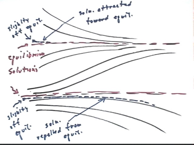
The figure below depicts the direction field for the equation

• dy/dt = -.1(y+2)(y-3)

Sketch a set of solution curves for this direction field.

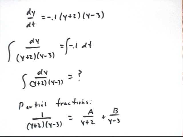
Solve the equation dy/dt = -.1(y+2)(y-3).

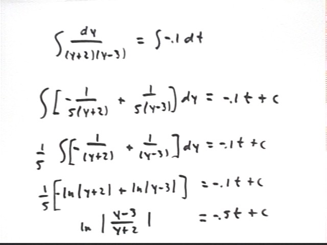
We easily separate variables to get

dy / [ (y+2)(y-3) ] = dt.

To integrate dy/ [ (y+2)(y-3) ] we use partial fractions:

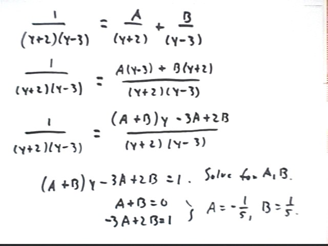
There exist A and B for which 1 / [ (y+2) (y-3) ] = A / (y+2) + B / (y - 3).

A / (y+2) + B / (y - 3) = [ A ( y - 3) + B ( y + 2) ]  / (y+2)(y-3).  Simplifying this expression we get

[ ( A + B ) y - 3 A + 2 B ] / (y+2)(y-3).

If

• [ ( A + B ) y - 3 A + 2 B ] / (y+2)(y-3) =  1 / (y+2)(y-3)

for all y then

• A + B = 0 and -3A + 2B = 1.

Solving for A and B we get

• A = -1/5, B = 1/5.

Thus

•  1 / (y+2)(y-3) = -1 / (5 (y+2) ) + 1 / 5(y - 3).

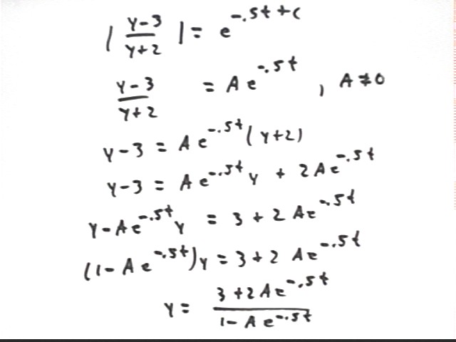
The solution (see details below; steps have been left out which should be familiar by this point) is

• y = (3 + 2 A e^-.5 t) / (1 - A e^-.5 t),

where A is any  nonzero constant.

Plotting this family of solutions, for A = -10 to A = 10, along with the direction field we get the following:

.

Remember that the logistic equation, often applied to population growth in environments with limited carrying capacity, is

dP/dt = k P (L - P),

where L is the population at carrying capacity.

Note that this is just a modification of the exponential growth equation

dP/dt = k P,

multiplying by the factor L - P, which approaches zero at P approaches carrying capacity. 

For small P our equation dP/dt = k P (L - P) gives us a pretty constant growth rate, since for small populations L - P is pretty close to L.  So we start with something very much like exponential growth. 

To solve this equation, we first separate variables to get

dP / [ P ( L - P) ] = k dt.

We solve this equation using partial fractions, just like in the preceding example.  Details are shown below.

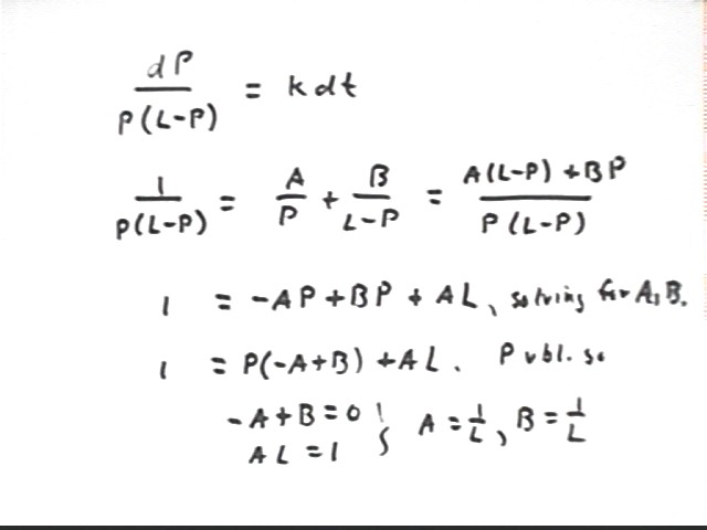
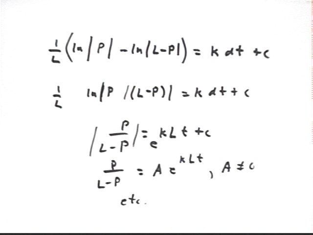
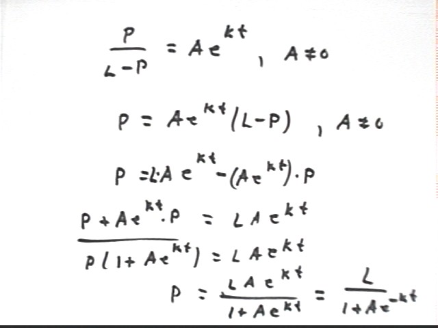
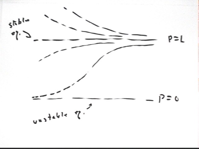
We end up with solution

P = L / (1 + A e^(-kt) ).

This function shows us that we have unstable equilibrium at 0, stable equilibrium at L.  That is, a small population moves away from the P = 0 equilibrium toward the stable equilibrium at P = L.

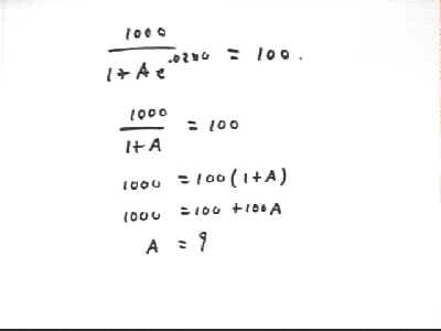
We can find the specific functions for a variety of different intial conditions.  For example if we know that the initial population is 100, carrying capacity is 1000 and the initial growth rate is 2% per unit of clock time then:

• The initial growth rate is k, so k = .02.
• At t = 0 the population is 100, so

P(0) = 1000 / (1 + A e^(.02 * 0) ) = 100.

We solve for A, obtaining  A = 9.

So P = L / (1 + A e^(kt) ) becomes

• P(t) = 1000 / (1 + 9 e^(-.02 t))

The direction field for this equation is shown below.  Note that the scale permits us to trace a solution curve from near the unstable equilibrium solution y = 0 to near the stable solution at y = 1000.

The solution obtained above for initial population y = 100 is shown with the direction field: