Annotated training algorithm

A neural net consists of a set of inputs, a 'black box' containing one or more adjustable parameters and a rule or set of rules for applying these parameters to the inputs. The rule that governs the behavior of the 'black box' is nonlinear with respect to the inputs.

A training set consists of a set of training inputs along with the ideal output(s).

To train the network the values of the parameters in the 'black box' are adjusted until the output that results from the training inputs is sufficiently close to the desired output.

Here we let X stand for the set of training inputs and Y for the ideal output, with C(0) a matrix of parameters:

X = set of training inputs
Y = ideal output
C(0) matrix of initial parameters

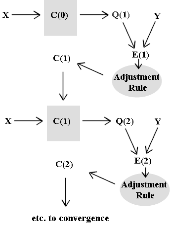
Oversimplified version:

An oversimplified schematic might be the one shown below, where training input X is fed into the 'black box' with parameters C(0), which yields output Q(0).

The output Q(0) is compared with the 'ideal output' Y to obtain error E(1).
This error is fed into the adjustment rule to modify the parameters of the 'black box', arriving at parameters C(1).
The training input X is again fed into the 'black box' and the process repeated, obtaining a second error E(2) which is used with the adjustment rule to obtain a new set of parameters C(2).

This process is iterated until the convergence criterion, whatever it happens to be for the specific process, is met.

* think of an example; Newton's Method for single-vbl fn ... **

Our model:

In the model we're going to consider here we break down the 'black box' into a set of 'neurons', each with a number of synapses. Each synapse of each neuron has a strength. Neuron strengths are the parameter in our matrices C( ).

X will stand for a set of N training vectors, each with m components. The ith vector will be denoted x(i), and its components x(i, j) with j running from 1 to m. Thus X can be represented by the N x m matrix depicted below.

We assume a number N of neurons equal to the number N of training vectors. The output of each neuron will be a single number y(i).

Our ideal output Y will be a vector consisting of N components y(i), as depicted below.

Each neuron will have m parameters, one for each component of an input vector. Thus C(0) can be represented for all neurons as an N x m as a matrix C(i,,j,0), with each column representing the parameters for a single neuron. The jth neuron will be represented by the jth column of this matrix:

In this model we will train one neuron at a time so we need not consider the entire matrix C(i, j, 0). We will denote the jth column of the matrix C(i, j, 0) by Cj (i, 0). This column vector will be modified with consecutive iterations to give us Cj (i, 1), Cj (i, 2), ..., Cj(i, k), ... .

The ith row of the X matrix corresponds to a single vector x(i, j), where j runs from 1 to m. We first consider the action of the first neuron on the vector x(i, j).

For simplicity we will assume that our neuron first simply multiplies the input row vector by the column vector consisting of its parameters, obtaining the sum

Sj x(i,j) * c1(j, 0) .

Repeating this for all N input vectors we obtain a row vector [ Sj x(i,j) * c1(j, 0), 1 <= i <= N ]

To each sum Sj x(i,j) * c1(j, 0) we apply a nonlinear transformation to obtain f1(i), obtaining the vector

Q(1) = [ f1(i), 1 <= i < = N ].

This vector is the output of the first neuron of our 'black box' corresponding to our input training matrix X and our initial parameters C1(j, 0). This vector is a vector in N-dimensional real space.

We will train our neurons one at a time. Each neuron will will act on the entire training set to produce output Q(i), where i is the number of the neuron, and will

contribute a basis vector R(i) to an orthogonal basis of N-dimensional real space,
incur an error vector E(n) orthogonal to the new basis vector or previous error vector or something

Our more specific procedure is represented by the schematic below:

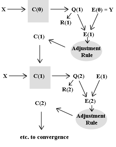
The motivation for this approach:

Our model might be such that it is difficult to approach the ideal output Y using a single neuron. There might be a tendency for the output of a single neuron to 'fall into bad habits', for example falling into a local minimum (converging to something but not to Y), or to oscillate around on some path that doesn't run very close to the local minimum.
Analogy: If you set a robot down in mountainous terrain and tell it to always go downhill it will get stuck at the lowest point of the first enclosed valley it encounters. If you give it a little more freedom than that it might end up endlessly circling the lowest point. More about this later.
If we can train the network in one linearly independent direction for each neuron we can avoid much of this behavior.

The vector Q(1) will be taken to be our first basis vector

R(1) = Q(1)

The initial error E(0) will be taken to by our ideal output Y.

We project the error E(0) on R(1). The scalar projection is

scalar projection = E(0) dot R(1) / || R(1) ||

and the vector projection is found by multiplying the scalar product by the unit vector in direction of R(1)

vector product = E(0) dot R(1) / || R(1) || * R(1) / || R(1) || = w1 R(1) with W1 = E(0) dot R(1) / || R(1) ||^2.

Our error vector is at this point E(1) = w1 R(1) - Y.

We adjust our parameters C1(j, 0) to try to reduce our error:

We regard each parameter C1(j, 0) as a variable influencing E(1).
We therefore need to calculate the rate at which E(1) changes with respect to each of the N parameters C1(j, 0)--i.e., the derivative of E(1) with respect to C1(j, 0) for each j.
Depending on the exact nonlinear function our neuron uses to obtain Q(1) we should be able to calculate these derivatives fairly easily.

What we end up with is the Jacobian of E(1) with respect to the parameter set C1(j, 0). This sounds pretty horrible but it's fairly straightforward, assuming our nonlinear transformation involves a function of which we can take derivatives (e.g., affine transformation, exponential functions, sigmoidal functions etc.). If not we could probably vary our parameters C1(j, 0) and see how E(1) changes, obtaining useful approximations.

We then penalize any parameter that tends to increase E(1) and reward any parameter that tends to decrease E1. We also avoid significant-figure errors by penalizing small R(1).

The specifics:

We need to calculate the rate at which E(1) changes with respect to each of the N parameters C1(j, 0)--i.e., the derivative of E(1) with respect to C1(j, 0) for each j.

A single input into a single neuron

let X stand for the set of training inputs and Y for the ideal output, with C(0) a matrix of parameters:

X = set of training inputs
Y = ideal output
C(0) matrix of initial parameters

Preliminary development in 3 dimensions.

We start with 3 input vectors, our 'training inputs', arranged here as rows in a matrix. Each vector in this example has dimension 4 so the matrix has dimension 3 x 4. However this dimension is arbitrary, as is the number of input vectors. We let X stand for the matrix and x, for the vectors:

training matrix: X = [x1, x2, x3, x4]T = [[x11, x12, x13, x14], [x21, x22, x23, x24],[x31, x32, x33, x34]].

In general our training matrix will be N x m, consisting of N training input vectors each of dimension m.

Each of the training inputs xi has an ideal output, which is a real number yi. Our output vector is therefore

Y = [y1, y2, y3]T,

represented here as a column vector.

In general if there are N training input vectors Y will be an n-dimensional vector.

We have a 'hidden layer' of N neurons, one for each training input vector.

Each neuron can be thought of as a 'black box' with m parameters which can be represented as a column vector [c1, c2, ..., cm] whose dimension matches that of a single input vector. These parameters are initially random within some appropriate range. To distinguish the parameters for one neuron from those for another we will use an additional subscript i corresponding to the number of the neuron: [ci1, ci2, ..., cim] is the current set of parameters for the ith neuron. These parameters correspond to synapses. ** For the current example m = 4. **

** it looks here as though we need three subscripts, one for the neuron, one for the position in the vector, one for the training level k. **

We will begin by training the first neuron. This is done through a series of iterations, with each iteration strengthening (increasing) or weakening (decreasing) each individual synapse depending on whether its effect is to move us toward or away from our goal. The training of this and of each subsequent neuron will cease when our output is considered to have converged--to have either stopped changing significantly or to have approached a given state to a prespecified level of precision.

We might therefore think of the synapses as being triply-subscripted variables cijk, with i standing for the number of the neuron, j for the position in the m-dimensional vector corresponding to that neuron, and k the number of the current iteration.

We will first think of training our first neuron and will simplify notation by denoting that neuron's parameters, or synapse strengths, as c1 =[ c11, c12, ..., c1n]. We note that the matrix X is compatible for multiplication by the column vector [c11, c12, ..., c1m].

To obtain the output of our first neuron we first use our randomly generated values of the c1j.

We find the product X c1 = [ S ( xij c1j) ] ** no--need n vectors in matrix--= x11 c11 + x12 c12 + ... + x1m c1m, ** with the summation taken over j and the components of the resulting vector indexed by i.

This gives us a vector of dimension N. T

To each component of this vector we apply the same nonlinear function F to obtain a vector Q = [ f1, f2, ...,f3], with fj = F(c1j).

** we might in applying the Gaussian use sum(xi - ci)^2 / (2 * std dev) **

We will use each of the three neurons in our three-input case to 'train' the output to minimize the component of the error in one of the three linearly independent directions of 3-dimensional space.

We might use a simple affine transformation of the product. We obtain X c1 = S ( xij c1j) and we simply add the arbitrarily chosen constant vector [1, 1, 1] to our result to obtain Q = [ S ( xij c1j) + 1 ]. Other common transformations include **

The details are not at this point important. However we should understand that our result Q will be a vector with 3 components, which we think of as represented with respect to a standard 3-dimensional Cartensian coordinate system, along with our ideal training output Y.

Since our parameters c1j were generated randomly it is not possible that Q will be equal to Y. We in fact expect that the magnitude and direction of Q will be unrelated to those of Y.

Let R1 = Q . We will minimize the error Q - Y in the direction of R1 .

We now project Y on Q , obtaining the vector projection ** use DERIVE **

Annotated training algorithm.

The My notation is a bit cumbersome but should be fairly obvious. My comments will often be obvious to you, but if they are correct they should be directly adaptable into code or pseudocode.

I also looked up some information on the conjugate gradient method of adjusting parameters, which adjusts the things in a set of mutually orthogonal directions to avoid possible oscillations of the solutions in a 'long, narrow well', where the curvature in one direction is much greater than in another, causing the parameters to bounce around off the closer walls and converge to the desired minimum very slowly. I don't have details I can probably figure out how to implement such a beast, but will confine comments here to the gradient descent method.

I've said more than you might need to just implement the thing, especially under the constraints of time. I've given a bit of the geometric interpretation, which might or might not be helpful to you. I can go into more detail there but didn't want to bog down the information about the implementation. Program from a room to

You start with an array of N training data, which consist of a set of N input vectors each of form X = [ x1, ..., xm }T, and a desired output y. The outputs form the N x 1 array Y.

Step 1

E0 = Y

Initialize the error vector as the desired output array.

Scale E0

I assumed that this means to give E0 some standard magnitude. The easiest way to do this would seem to be to replace E0 by E0 / || E0 ||, where || E0 ||^2 is the Pythagorean magnitude, the sum of the squares of the elements of E0, designated in the article as the product of the transpose of E0 and E0.

Initialize C1 as C(1,0)

C(1,0) = [ c1, c2, ..., c(m+1)], where m is the number of input neurons and c(m+1) is the standard deviation term of the radial activation function.

k = 0

Repeat

Calculate Q1

Apply the activation function phi to each of the N input vectors, using the m+1 parameters of C(1,k). The exponent for each will be sum( (xi - ci)^2 ) / c(m+1)^2. This gives you the N x 1 array Q1.

R1 = Q1

This is the first of the set of orthogonal vectors which will form a basis for the error space.

w1 = E0T * R1 / || R1 ||^2

Very straightforward calculation.
The idea here is that ideally the output w1 Q1 will match the desired output Y. E0T * R1 / || R1 || is the magnitude of the vector projection of E0 on R1. This makes the product w1 Q1 for the current value of Q1 match Y.

C(1, k+1) = C(1,k) - correction term

The correction term depends on the method used. For the gradient descent method we want this term to be proportional to the rate at which the squared magnitude || En ||^2 of the error changes with respect to the present array C1 of parameters. We add a term proportional to 1 / || R1 ||^2 to compensate for the effect of small values of || R1 ||. This gives the vector J1, whose rate of change we calculate.
The correction term is a constant multiple of the rate of change dJ1 / dC1 of the J vector. The constant is `eta (which for efficiency in some cases might be dependent on the 'time' k or the status of convergence).
The derivative of J1 is easily calculated from the derivative of Q1. Since Q1 is an array of values given by the activation function, dQ1 / dC1 is easily calculated using first-semester calculus (chain rule). dQ1 / dC1 is an m+1 x N array (eqn 30 in the article). R1 is an N x N array. R1 R1T is an N x N array and R1T R1 = || R1 ||^2, simply a number. The jth column of R1 R1T is, unless I'm seriously mistaken, equal to the product of the jth element of R1 and the N x 1 column vector R1.

k = k + 1

Until Convergence

I assume that you know what statistical measure of convergence is appropriate. The article provides no guidelines here, and I imagine that some trial and error would be necessary to adjust the efficiency of the algorithm.

Test the network on testing data

The testing data is your baby, obviously dependent on the specific situation.

Check stopping criteria

The AIC formula is self-explanatory. You might know of other criteria.

If adequate, stop

Else, proceed to next step.

Step n

Scale E(n-1)

Replace E(n-1) by E(n-1) / || E(n-1) ||.

Initialize Cn as C(n,0)

just another randomized array with m+1 elements in the appropriate range

k = 0

Repeat

Calculate Qn

Again apply the activation function, with current values of Cn, to training vectors X.

`alpha(i,n) = RiT Qn / || Rn ||^2

For each existing Ri, this calculates the multiple of Ri which represents the component of Qn in the direction of Ri.

Rn = Qn - sum(`alpha(i,n) Ri)

We simply subtract from Qn the components of Qn in the directions of the Ri, leaving Rn, which is the component of Qn orthogonal to all the existing Ri vectors.
This works because all the Ri are orthogonal.

wn = E(n-1)T * Rn / || Rn ||^2

Ideally the output wn Qn will match the desired output Y. E(n-1)T * Rn / || Rn || is the magnitude of the vector projection of E(n-1) on Rn. This makes the product wn Qn for the current value of Qn match Y.

C(n,k+1) = C(n,k) - correction term

Again a straightforward calculation for gradient descent (see analogous step in initial loop).

k = k + 1

Until Convergence

En = E(n-1) - wn Rn

Straightforward calculation of new error term, the component of the old error orthogonal to the new Rn.

test, check, etc.