Class Notes 101117

Question from student: How do we deal with a a 6 degree angle with horizontal?

Answer:  It depends on the situation. 

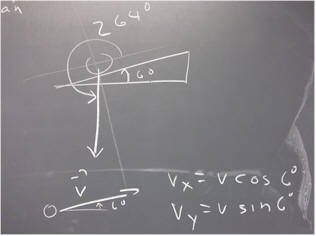
For example if the context is an incline at 6 degrees, then we rotate the x and y coordinate axes so the x axis is parallel to the incline.  If the incline is up and to the right, the angle of the weight vector is then 264 degrees with respect to the positive x axis.   We find its components using the cosine and sine function (x component is weight * cos(264 deg) and y component is weight * sin(264 deg) ).  If the incline is up and to the left then the angle is 276 degrees.

If the context is a velocity vector (or any other vector directed at 6 degrees), then if the x axis is horizontal the angle of the vector with respect to the positive x axis is either 6 degrees (vector at 6 degrees above horizontal, directed up and to the right), 174 degrees (6 degrees above horizontal directed to the left), 354 degrees or 186 degrees (directed 6 deg below horizontal and to the right or to the left, respectively).   If theta is the angle, the components are v cos(theta) and v sin(theta).  In the figure below we sketch the 6 degree case and give the components.

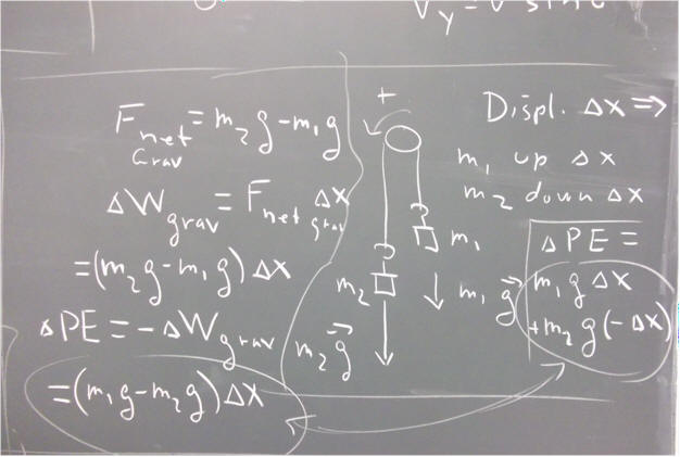
PE and Atwood machine:

If masses m1 and m2 are hung on opposite sides of a light frictionless pulley, then gravity exerts forces m1 g and m2 g.  Choosing counterclockwise as the positive direction, a positive displacement `dx gives m1 a vertical displacement of + `dx and m1 a vertical displacement of - `dx, resulting in a net PE change of m1 g `dx - m 2 g `dx.

Alternatively, the net gravitational force on the system is m2 g - m1 g.  The work `dW_grav done by this force on the system is therefore (m2 g - m1 g) `dx.  This is the work done by the gravitational force, which is conservative.  The change in gravitational PE of the system is therefore equal and opposite to this work so that

`dPE_grav = - (m2 g - m1 g) `dx = m1 g `dx - m2 g `dx,

in agreement with our previous result.

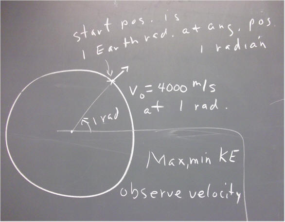
Orbital simulation:  How do we do the 'straight shots' with initial velocities 4000 m/s, 5000 m/s, etc..?

Answer: 

The starting position will be defined by the 'initial angular position' and the 'initial distance'.  That position is shown below for initial distance 1 (corresponding to 1 Earth radius, i.e., to a point on the surface of the Earth) and angular position 1 (for 1 radian). 

The direction of a 'straight shot' is directly away from the center of the Earth, so the direction of the impulse must match the initial angular position.  In this example that would be 1 radian.  The initial velocity is numerically equal to the initial impulse.

So in summary, for the example below:

• Initial angular position is 1 radian.
• Initial distance is 1 Earth radius.
• Impulse of the 'burn' is 4000 (meaning 4000 kg m/s, on a 1 kg mass).
• Direction of impulse is 1 radian.

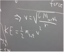
Question:  How to get the kinetic energy?

Answer:  You are asked for the kinetic energy per kilogram of the satellite's mass.  That will be 1/2 m v^2, where v is the speed in meters/second and m is 1 kg.

You can observed the speed in the box just above the 'Run (don't clear)' button.  You can watch how the speed changes and click the 'pause simulation' button when you see the speed hit its max or min value for a given orbit.

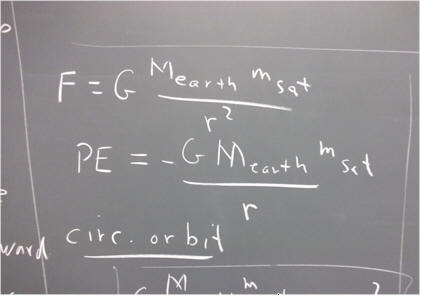
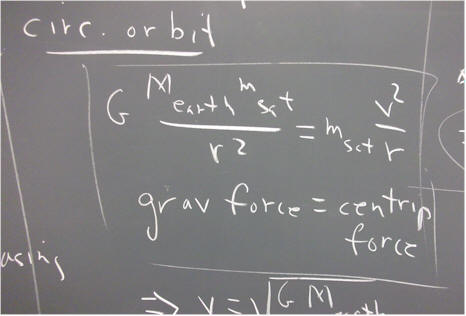
Below is a summary of what you know about gravitation:

• F = G M_earth m_satellite / r^2 is the force between Earth and satellite.
• PE = - G M_earth m_satellite / r is the PE of the satellite relative to infinite separation.  Note that PE is always negative, so that a greater separation r leads to a larger denominator which leads to a result of smaller absolute magnitude.  However that result is negative, and since a negative quantity of smaller magnitude is greater, the PE increases with increasing separation.
• For a circular orbit the gravitational force is equal to the centripetal force.  Since centripetal acceleration is v^2 / r, the centripetal force on the satellite is m_satellite * v^2 / r.  The condition for a circular orbit is therefore

-G M_earth m_satellite / r^2 = m_satellite v^2 / r.

This equation is easily solved to yield v in terms of r.  We get v = sqrt( G M_earth / r).

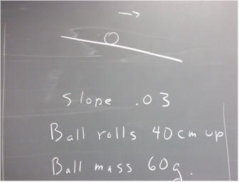
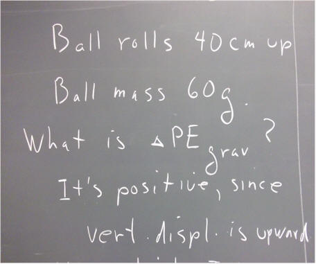
A bell of given mass rolls the given distance up an incline, whose slope is also given.

We wish to analyze the potential energy change.

We make the following observations about the PE:

`dPE is positive, for each of the following reasons:

• the ball moves further from the center of the Earth
• the vertical displacement of the ball is upward
• the component of the gravitational force parallel to the incline is down, while displacement is up the incline, so that gravity does negative work on the ball, resulting in a positive change in gravitational PE

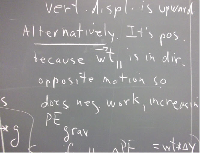
More specifically

• `dPE_grav = weight * `dy = (.06 kg * 9.8 m/s^2) * 40 cm = .59 N.

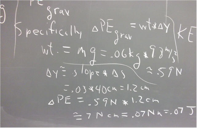
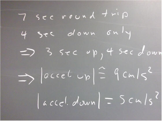
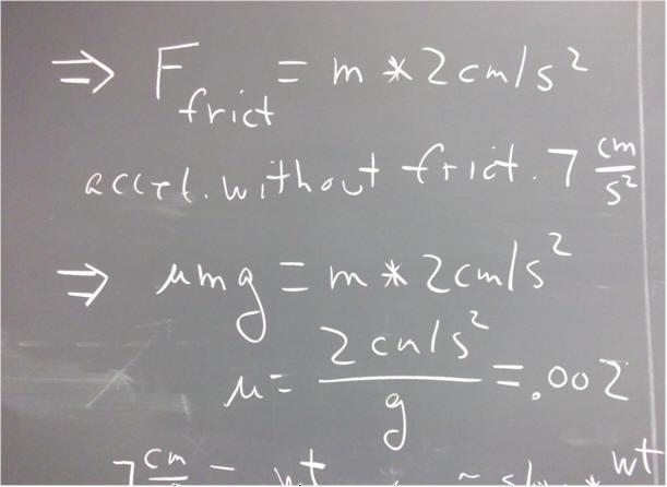
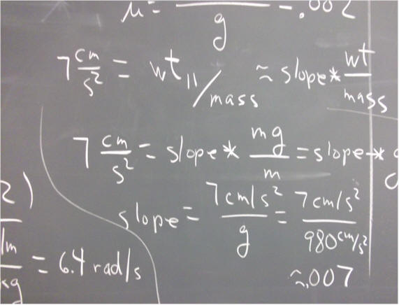
If a ball on a ramp requires 7 seconds for a round trip up to the 40 cm mark and back, and 4 sec for the trip back, then the magnitude of its accelerations up and down are about 9 cm/s^2 and 5 cm/s^2.

• The 4 cm/s^2 difference is due to double the force of rolling friction, which is therefore mu * weight = mu m * g = m * 2 cm/s^2, where m is the mass of the ball.  Thus mu = 2 cm/s^2 / g = 2 cm/s^2 / 980 cm/s^2 = .002.
• The mean acceleration 7 cm/s^2 is the acceleration due to the slope of the ramp.  Since the parallel component of the weight of the ball is approximately equal to slope * weight, we have slope * m * g = m * 7 cm/s^2, so that slope = 7 cm/s^2 / g = .007.

SHM occurs when F_net = - k x, and is characterized by omega = sqrt(k/m).  The reference-circle model applies, as introduced previous and as sketched below.  If theta = 0 when t = 0, then at clock time t

• The angular position is omega * t.
• The x coordinate is x = A cos(omega * t), where A is the amplitude of motion.
• The velocity and centripetal acceleration vectors have magnitude omega * A and omega^2 * A, and are directed at angles theta + 90 deg and theta = 180 deg. 
• The maximum velocity and acceleration of an object whose position is the x coordinate are respectively equal to the reference-circle speed and centripetal acceleration omega * A and omega^2 * A.
• Their x components are therefore v_x = omega * A * cos( omega * t + 90 deg) and v_x = omega^2 * A * cos(omega * t + 180 deg).  These components can be expressed in terms of the angle omega * t as - omega * A * sin(omega * t) and -omega^2 * A * cos(omega * t).

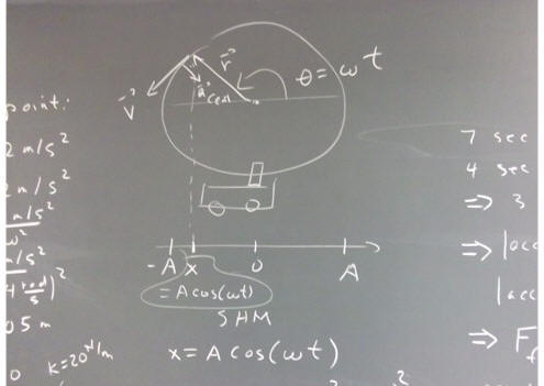
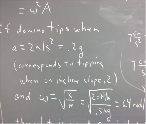
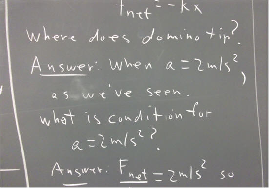
We apply this to the tipping of a domino resting in a cart.  It has been observed that the domino tips when the acceleration of the cart is 2 m/s^2, or about .2 g's.  The cart and suspended dominoes have a total mass of roughly .5 kg, and the rubber band chain used here exerts a force approximately equal to F = - k x, where k = 20 N / m.

omega = sqrt( k / m ) = 6.4 rad/s, as shown below.  6.4 rad is slightly more than 1 revolution or 1 cycle, so we expect the cart to oscillate with a period slightly less than 1 second.

If the cart is released at position A with respect to equilibrium, the domino will or will not tip, depending on the value of A.  We observe that the domino doesn't tip when A = 3.5 cm, but does tip when A = 4.0 cm.

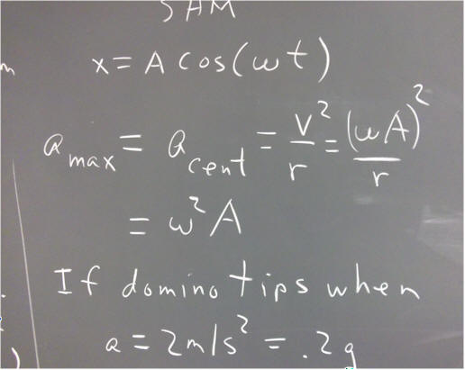
Assuming the motion to be simple harmonic, the maximum acceleration a_x = omega*2 * A should occur at the extreme points of the motion (a_x = - omega^2 * A cos(omega * t), which is maximized when | cos(omega * t) | = 1, which is the maximum magnitude of the cosine function; the position x = A cos(omega * t) is also maximized when | cos(omega * t) | = 1; so acceleration is maximized when position is maximized).

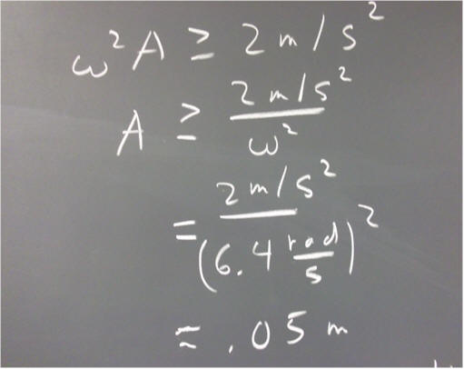
Thus the domino should tip when omega^2 * A >= 2 m/s^2.

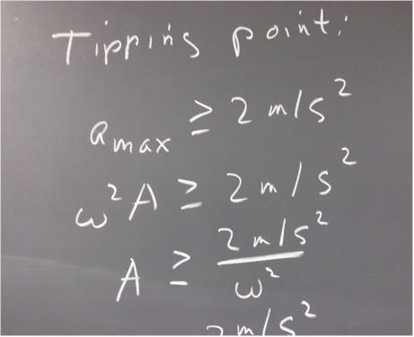
The equation omega^2 * A >= 2 m/s^2 is easily solved, as shown below.  We find that tipping should occur according to the condition A > = .05 m, or 5 cm.  If A < .5 cm, tipping should not occur.

The observed cutoff for tipping was a bit lower than A = 4 cm.  Our results are roughly, but not exactly, equal to the prediction.

Depending on the accuracy of our estimated parameters m = .5 kg and k = 30 N / m, we might or might not regard the level of agreement as an indication of consistency.

If refined measurements don't indicate consistency, then it is possible that the motion is not all that close to simple harmonic in nature.  This would imply that our force is not exactly a linear function of position over the observed range of motion.

We could also ask the question based on our observed parameters k = 20 N / m, mass = .5 kg.

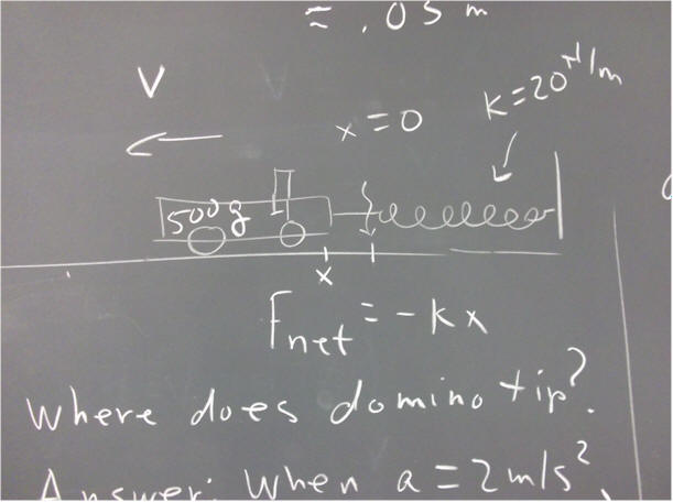
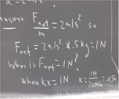
The condition for a = 2 m/s^2 is that F_net / m = 2 m/s^2.

If m = .5 kg, then F_net / m = 2 m/s^2 implies that F_net = 1 N, as indicated below.

If F_net = k x, then x = F_net / k = 1 N / (20 N / m) = .05 m, or 5 cm.

This agrees exactly with the prediction of our simple harmonic motion model.  This shouldn't be all that surprising, since that model was based on the same parameters (k = 20 N/m and mass = .5 kg).

University Physics Supplemental Notes

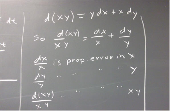
d(xy) is the differential of x y.  It is equal to y dx + x dy.

The implication is that if an observed value of x is considered uncertain by amount `dx, and our value of y by `dy, our value of x * y should be considered uncertain by the amount y `dx + x `dy.

The uncertainty in x * y is d(x y), which is the proportion d(x y) / (x * y) of the value of x * y.  We call this the proportional uncertainty in x * y, or alternatively the proportional error in x * y.  If we multiply this by 100% we get the percent uncertainty in the value of x * y.

A simple step shows that d(x * y) / (x * y) = dx / x + dy / y. 

• dx / x is the proportional uncertainty in x
• dy / y is the proportional uncertainty in y

We draw the following conclusion:

The proportional uncertainty in x * y is the sum of the proportional uncertainties in x and in y.

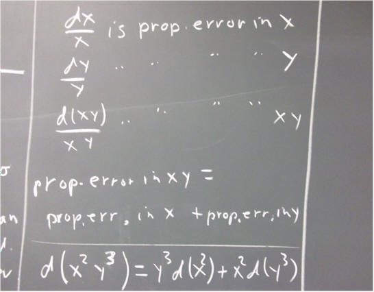
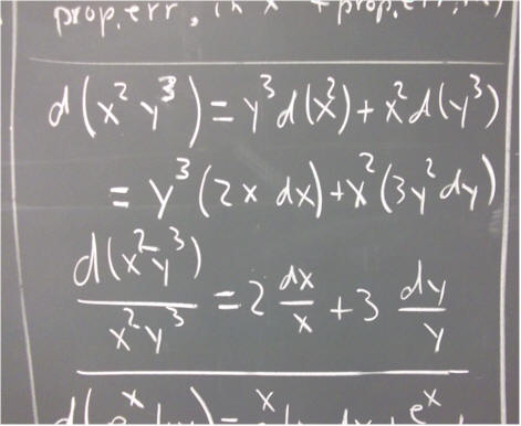
It is suggested that you perform a similar analysis of the expression x^2 * y^3. 

The results are shown below.  We can summarize the final result as follows:

The proportional uncertainty in x^2 * y^3 is double the proportional uncertainty in x, added to triple the uncertainty in y.

If v0 = 0 then the acceleration of an object which starts at x = 0 when t = 0 is a = 2 x / t^2.

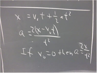
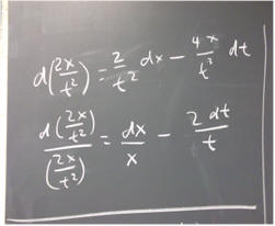
The differential of this expression is shown in the first step below, and the proportional uncertainty in the second.

Our conclusion:

When a is determined by measurement of the displacement x, from rest, in a time interval of duration t, the proportional uncertainty of the result is the sum of the proportional uncertainty in x, and double the proportional uncertainty in t.

The result looks like a subtraction and not an addition, and in fact it is.  However the uncertainties dx in x and dt in t each indicate a possible deviation in either the positive or the negative direction, so either could be positive and either could be negative.  This illustrates another principle:

When the expression for the proportional uncertainty in a quantity is a sum of a two or more terms, the proportional uncertainty is the sum of the magnitudes of those terms.

Quick summary of normal distributions:

When a large number of observations of a quantity are taken to sufficient precision, the results will tend to vary about some mean value.  Normally, if the observations are unbiased, they will tend to follow a certain distribution, appropriately called the normal distribution.  This distribution is a probability distribution.  You should be familiar with probability distributions from your study of applications of the integral in first-year calculus.  If not, you should look up the term, as explained from a calculus-based viewpoint.

The normal distribution is the limiting case of the binomial distribution, and the number n of occurrences approaches infinity.

The standard deviation of a set of observations is basically the square root of the mean value of the squared deviations of the observed quantities from their mean.  Think first of the average of the deviations of the numbers from their mean, which provides a measure of how 'spread out' the observations are.  For reasons related in a fairly straightfoward way to the binomial distribution, however, it is the standard deviation rather than the average deviation that defines the normal distribution.

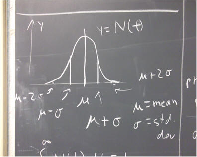
If the mean is indicated by mu and the standard deviation by sigma, then a graph of the normal distribution is as depicted below.  The t value t = mu is the center of the distribution, the mean, and the distribution is symmetric with respect to mu.  The t value t = mu + sigma is the value which lies 1 standard deviation 'above' the mean, and t = mu - sigma is one standard deviation 'below' the mean.  The descriptions of t = mu + 2 sigma and t = mu - 2 sigma should be obvious.

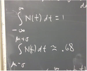
Being a probability distribution, the integral of the normal distribution, over all possible values of t, must be 1.  This corresponds to the fact that the probability of something happening is 100%, or 1.  The integral over all values of t is the probability that one of these values will be observed.

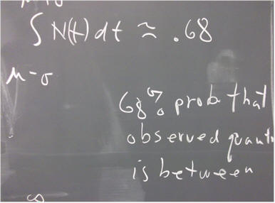
The probability of an occurrence within one standard deviation of the mean is just the integral of N(t) over the corresponding interval, which runs from t = mu - sigma to t = mu + sigma.  This integral cannot be evaluated exactly, but can be approximated to any desired degree of precision.  To 2 significant figures the probability is .68, or 68%.  In a large number of normally distributed set of observations, about 68% will lie within 1 standard deviation of the mean.

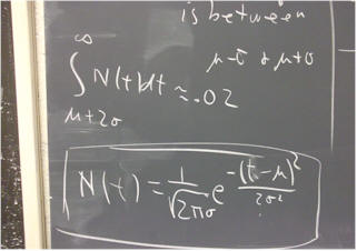
The normal distribution function can be expressed in terms of mu and sigma, as the exponential of a negative square:

• N(t) = 1 / ( sqrt(2 pi) ( sigma) ) * e^(-(t - mu)^2 / (2 sigma^2) ).

The normal distribution for mu = 0 and sigma = 1 is plotted below.

You should estimate the area beneath the curve and verify that it is reasonably close to 1.

The function for mu = 0 and sigma = 1 is simple enough:

N(t) = 1 / sqrt(2 pi) e^(-t^2 / 2)

The t = 0 value is easy to estimate:

sqrt( 2 pi ) = sqrt( 6.28 ).  2.5^2 = 6.25, so sqrt( 2 pi ) is close to 2.5.  1 / sqrt(2 pi) is therefore close to 1/ 2.5 = .4.

If t = 0, then we get 1 / sqrt( 2 pi ) e^0 = 1 / sqrt( 2 pi ) * 1 = .4, approximately.

You should check to be sure this is consistent with the graph as depicted above.

You should be able to make this estimate any time, mentally, without resorting to your calculator.

You should plug t = -3, -2, -1, 0, 1, 2, 3 into your calculator and verify that the resulting values correspond to the above graph.

The graph below includes vertical lines at 1, 2 and 3 standard deviations from the mean.

The areas of the corresponding regions under the graph are about 34%, 14% and 2% of the total area under the curve.  You should make estimates sufficient to satisfy yourself that it is so.

You should also use the values you obtained for t = 0, 1, 2 and 3 to evaluate the areas of the trapezoids in the graph as shown below, and compare to the 34%, 14% and 2% figures given previously: