Class Notes 100920
Notes from class have been added. Further revisions are possible, but this can be regarded as a complete document.
University Physics students should note the importance of being able to reason out problems using basic definitions, as well as the efficiency and insight gained from combining such reasoning with symbolic solutions.
Text Assignment
General College Physics:
Chapter 2 Problems you should read carefully and sketch out how you will solve them, what you do and do not understand about them, etc.
1-5, 6, 9, 11, 16, 22, 27
34, 37, 43, 52, 55, 58, 63
Also you should read Chapter 4, Sections 1-6.
University Physics:
Assigned Chapter 2 Problems are as listed below. You should sketch out how you will solve these problems, using direct reasoning to the greatest possible extent. Then you should sketch out how to perform the more general symbolic solution. Naturally I won't be surprised if I get specific questions on some of these problems.
54, 57, 60, 63, 66
72, 77, 82, 87, 90
Also read through Chapter 4, Sections 1-5
Important Resources for Test Preparation: Introductory Problem Sets and other recommended resources:
There will soon be a test, entitled the Major Quiz. You can check out tests at the link http://vhmthphy.vhcc.edu/tests/ . More details on testing, in class Wednesday.
At the Assignments page for distance students(http://vhcc2.vhcc.edu/ph1fall9/frames_pages/assignments.htm) you will see the following:
In some of Assignments 1-8, there are Randomized Problems. The first couple include instructions. These problems are of the same form as many problems that occur on the Major Quiz, so it is recommended that you submit any of these problems that aren't completely obvious to you, using the same procedures you have used to submit other documents. Insert your responses in the appropriate places. I do ask that you mark insertions before and after with #### so I can quickly locate them, but these are short documents and if you happen to forget it won't be a big deal.
Also you will see the link http://vhmthphy.vhcc.edu/ph1introsets/default.htm, which is a link to the Introductory Problem Sets. You should take a quick read through Sets 1 and 2, just to see what's there. Ideally you will understand every problem, and will understand completely the explanations given in the provided solutions, generalized solutions, and figures.
The Introductory Problem Sets are designed to stand alone as an introduction to very basic problems and procedures. One important thing, from your perspective, is that after the Major Quiz, problems from the Introductory Problem Sets frequently appear on tests.
Energy in the two-magnet system, experiment with coasting car
Substituting a = F_net / m into the fourth equation of motion leads to the definitions of work and kinetic energy, and the work-kinetic energy theorem. Substituting a = F_net / m into the second equation of motion leads to the definitions of impulse and momentum, and the impulse-momentum theorem.
The energy to push the magnets together came from the Cheerios I theoretically ate for breakfast (note the energy conversion is only about 15% efficient).
The work done by the force I exerted goes into the potential energy of the magnet system. When I release the car, the energy is mostly transformed into KE, though some is lost to friction before the magnetic force becomes insignificant.
When the system is first released the magnitude of the force of repulsion between the two magnets exceeds that of the frictional force, and the car accelerates forward. The magnetic force decreases as the separation increases. At a certain point the magnitude of the magnetic force has fallen to the extent that it is equal to the magnitude of the frictional force, at which point the net force on the car and hence its acceleration is zero. Beyond this point the frictional force exceeds the magnetic force and the acceleration of the system becomes negative, so that the KE reaches its maximum at the point where the two forces are equal and opposite. (University Physics students should be able to explicitly relate this to the First Derivative Test). The car will then slow in response to the frictional force, its KE being gradually depleted as the car does work against friction. The car eventually comes to rest.
Units of force and work
F_net = m a. So the unit of a force is the product of a mass unit and an acceleration unit.
Units of mass include grams, slugs, kilograms and many others. Units of acceleration (being units of distance divided by squared units of time) include meters / second^2, miles / hour^2, (miles/hour) / second, kilometers / year^2 and many others.
Possible units of force would therefore include gram * meters / second^2, slug * kilometers / year^2, etc..
The work done by frictional force, for a given interval, is
The unit of work is therefore equal to the product of the unit of force and the unit of displacement.
Meaning of midpoint clock time
Suppose we have the following angular position vs. clock time data:
| clock time (counts) | angular pos (degrees) |
| 1 | 0 |
| 11 | 180 |
| 30 | 360 |
This data gives us two intervals. How long does the first last, and how long does the second?
A typical answer for the first is that it lasts 11 counts, while the second lasts 19 counts.
Another question: What is the count at the midpoint of the first interval?
A frequent answer is 5. However 5 is closer to 1 than to 11, so it isn't halfway. And 6 is closer to 11 than to 1.
Similarly we quickly see that the halfway clock time for the second interval is (11 + 30) / 2 = 20.5. You can (and should) easily verify that this is equally close to 11 and 30.
Now we ask about the table of average rate of change of angular position vs. midpoint clock time.
We easily see than during the first interval the angular position changes by 180 deg, during an interval that lasts 10 counts, so the desired average rate is 18 deg / count.
Similarly during the second interval the the angular position changes by another 180 deg, during an interval that lasts 19 counts, so the desired average rate is 180 deg / (19 counts) = 9.5 deg / count.
So our midpoint clock times are 5.5 counts and 20.5 counts, our average angular velocities 18 deg / count and 9.5 deg / count.
Our table is therefore as follows:
midpt clock time (counts) roc of angular pos wrt clock time (degrees/sec) 5.5 18 20.5 9.5 The logic of this table is simple enough. The average velocity on an interval typically occurs near (though usually not precisely at) the midpoint clock time. So this table is a reasonable representation of angular velocity vs. clock time.
We could easily construct a graph of this information, giving us a good approximation of a graph of the actual angular velocity vs. clock time graph.
Meaning of Tangent Line, Interpretation
After doing several trials, observing coasting distance vs. initial separation, we obtained a graph of coasting distance vs. separation. The graph might look much like the one below, with the points indicating data points, with a smooth curve sketched to fit the data points.
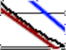
The figure below shows the same curve, with two line segments added.
The graph is of course not completely smooth, having been constructed of pixels. The figure below 'zooms in' on a small segment of the curve. Because of the jaggedness, the picture doesn't allow us to pinpoint exactly where the line segment actually touches the curve, but we have a pretty good idea. The actual point where the straight line segment just 'kisses' the curve is called the point of tangency.
As we can see from this picture, the curve is pretty nearly straight in this neighborhood of the point of tangency, with only slight curvature visible. The closer we are able to zoom in, the straighter the curve will appear.
It should be obvious that the slope of the curve, in a small neighborhood of the point of tangency, will vary little within that neighborhood, and will be very close to the slope of the tangent line.
It should also be obvious that if we construct chords over smaller and smaller intervals containing a specific point, the slopes of those chords get closer and closer to the slope of the tangent line. (University Physics students will recognize the application of limits to this description, and to the definition of the tangent line).
We therefore say that the slope of a curve at a point is the slope of its tangent line at that point (assuming that the curve actually has a tangent line at the point; this isn't the case for every possible curve, but it will be for most of the curves we use in this course).
Remember that the slope of either a chord or a tangent line is defined to be the rise/run between two points of that line. Any two points of a straight line will give you the same slope.
Masses rotating on a strap (important for University Physics, worth understanding but not essential for General College Physics)
For a magnet on a rotating strap, some points of the magnet are closer to the axis of rotation than others. The closest point is moving more slowly than the furthest, and the point halfway between the two is moving at a speed which is the average of the speeds of these two points.
A gram of the magnet at the closest point therefore has less KE than a gram of the magnet at the furthest point (of course the amount of magnet at a point is zero, since a point has zero volume, but let's not split those hairs just yet). If asked to compare these values with the KE of a gram at the midpoint, the first response would typically be that since the speed at the midpoint is halfway between the other two, the KE at the midpoint would also be halfway between the other two.
However it can't be so, since KE is proportional to v^2, not to v, and v^2 is not linear with respect to v.
The advantages of calculating in symbols (essential for University Physics, recommended for General College Physics)
You were asked in an earlier assignment to find values of vf for an object traveling a fixed distance on a ramp with a fixed acceleration, but for different values of v0, and to look for patterns.
The calculation is simple enough, using the fourth equation of motion.
In this case there is very little difference in the amount of work necessary to obtain the solutions. Were we plugging a lot of values into the fourth equation to solve for, say, the acceleration, it should be clear that we would be better off solving the equation symbolically then plugging in our numbers, rather than plugging them in at the beginning and solving the equation separately for each set of values.
This illustrates at least two advantages of solving in symbols. You get a formula which can be used for multiple sets of data, and it's just plain neater to solve using symbols than to fool with all the numbers and units through all the steps of the solution.
An additional, and greater, advantage is that the symbolic solution can be interpreted so that the effects of changing different quantities can be seen and understood in terms of the symbols, without the need to calculate results for multiple sets of data.
For example the expression vf = sqrt(v0^2 + 2 a (x - x0)) can be interpreted as a function of v0, with fixed values of a and (x - x0). Given sufficient knowledge of mathematical analysis, we can gain a lot of insight into, say, the problem of ordering v0, vf, v_mid_x, v_mid_t and `dv.
You should get in the habit of performing, thinking about and analyzing symbolic solutions so you can learn what they have to tell you.
extends from the closest to the furthest point of the magnet relative to the axis of rotation.
... force diagram for car-magnet system in different states; vel and accel diagrams ... opposite cars will exhibit a very nearly elastic interaction ...
... qa's for cal1? ...
frictional force resisting the car's forward motion becomes equal
Experiments
Questions related to experiments are denoted with `qx. Most of the questions for this assignment are related to experiments.
For the magnets on the rotating strap:
`qx001. How fast was each of the magnets moving, on the average, during the second 180 degree interval? All the magnets had the same angular velocity (deg / second), but what was the average speed of each?
****
#$&*
`qx002. For each magnet, one of its ends was moving faster than the other. How fast was each end moving, and how fast was the center point moving?
****
#$&*
`qx003. What was the KE of 1 gram of each magnet at its center, at the end closest to the axis of rotation, and at the end furthest from the axis of rotation?
****
#$&*
`qx004. Based on your results do you think the KE each magnet is greater or less than the KE of its center?
****
#$&*
`qx005. Give your best estimate of the KE of each magnet, assuming its mass is 50 grams.
****
#$&*
`qx006. Assuming that the strap has a mass of 50 grams, estimate its average KE during this interval.
****
#$&*
`qx007. (univ, gen invited) Do you think the KE of 1 gram at the center of a magnet is equal to, greater or less than 1/2 m v_Ave^2, where v_Ave is the average velocity on the interval?
****
#$&*
For the teetering balance
`qx008. Was the period of oscillation of your balance uniform?
****
#$&*
`qx009. Was the period of the unbalanced vertical strap uniform?
****
#$&*
`qx010. What is the evidence that the average magnitude of the rate of change of the angular velocity decreased with each cycle, even when the frequency of the cycles was not changing much?
****
#$&*
For the experiment with toy cars and paperclips:
`qx011. Assume uniform acceleration for the trial with the greatest acceleration. Using your data find the final velocity for each (you probably already did this in the process of finding the acceleration for the 09/15 class). Assuming total mass 100 grams, find the change in KE from release to the end of the uniform-acceleration interval.
****
#$&*
For the experiment with toy cars and magnets:
`qx012. For the experiment with toy cars and magnets, assume uniform acceleration for the coasting part of each trial, and assume that the total mass of car and magnet is 100 grams. If the car has 40 milliJoules of kinetic energy, then how fast must it be moving? Hint: write down the definition of KE, and note it contains three quantities, two of which are given. It's not difficult to solve for the third.
****
#$&*
`qx013. Based on the energy calculations you did in response to 09/15 question, what do you think should have been the maximum velocity of the car on each of your trials? You should be able to make a good first-order approximation, which assumes that the PE of the magnets converts totally into the KE of the car and magnet.
****
#$&*
`qx014. How is your result for KE modified if you take account of the work done against friction, up to the point where the magnetic force decreases to the magnitude of the (presumably constant) frictional force? You will likely be asked to measure this, but for the moment assume that the frictional force and magnetic force are equal and opposite when the magnets are 12 cm apart.
****
#$&*
`qx015. If frictional forces assume in the 9/15 document were in fact underestimated by a factor of 4, then how will this affect your results for the last two questions?
****
#$&*
`qx016. What did you get previously for the acceleration of the car, when you measured acceleration in two directions along the tabletop by giving the car a push in each direction and allowing it to coast to rest?
****
#$&*
`qx017. Using the acceleration you obtained find the frictional force on the car, assuming mass 100 grams, and assuming also a constant frictional force.
****
#$&*
`qx018. Based on this frictional force
How long should your car coast on each trial, given the max velocity just estimated and the position data from your experiment?
... this could be done with an inclined air track ...
... collision: release two cars simultaneously, one carrying two magnets and the other carrying one
****
#$&*
The following questions are for university physics students, though all but one are accessible to general college physics students, who are invited but by no means required to attempt them. Questions of this nature will be denoted by (univ; gen invited). Questions which actually require calculus are denoted (univ; calculus required). General College Physics students with a calculus background are invited to attempt these questions.
`qx019. (univ; gen invited) Looking at how v0 affects vf, with numbers: On a series of trials, a car begins motion on a 30 cm track with initial velocities 0, 5 cm/s, 10 cm/s, 15 cm/s and 20 cm/s. By analyzing the first trial in the standard way, the acceleration is found to be 8 cm/s^2. Using the equations of uniformly accelerated motion, find the symbolic form of the final velocity in terms of the symbols v0, a and `dx. Then plug the information common to all trials into this equation (i.e., plug in the values of `ds and a) to get an expression whose only unknown quantity is v0. Finally plug your values of v0 for the various trials into your expression, and obtain your values for vf. Sketch a graph of vf vs. v0 and explain as best you can, in terms of your direct experience with these systems, why the graph has the shape it does.
****
#$&*
`qx020. (univ; gen invited) Use your calculators to graph vf vs. v0, using the expressions into which you plugged your values of v0, and verify your graph.
****
#$&*
`qx021. (univ, calculus required) Should the derivative of vf with respect to v0 be positive or negative? Don't answer in terms of your function, your graph or your results. There is a good common-sense answer based on the behavior of the system and the nature of uniform acceleration.
****
#$&*
`qx022. (univ; calculus required) What is the derivative of vf with respect to v0? What does this derivative function tell you about the behavior of the system?
****
#$&*
`qx023. (univ; gen invited) Using the velocity and position functions for uniform acceleration, and the resulting equations of uniform acceleration, can you get an expression for the time required to achieve velocity v_mid_x in terms of v0, a and `dx?
****
#$&*
`qx024. (univ; gen invited) Using the velocity and position functions for uniform acceleration, and the resulting equations of uniform acceleration, can you get an expression for the velocity v_mid_t in terms of v0, a and `dx?
****
#$&*
`qx025. (univ; gen invited) Can you interpret the expressions for v_mid_x and v_mid_t to answer at least some of the open questions associated with the ordering of v0, vf, `dv, v_mid_x, v_mid_t and v_ave? Can you develop expressions that can be interpreted in order to answer the remaining questions?