Calculus II
Class Notes, 9/13/99
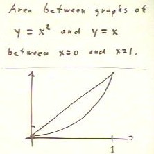
We wish to find the area between the graph of y = x^2 and
y = x, between x = 0 and x = 1.
We can do this in one of two ways.
- We can find the area under the higher curve, and the area
under the lower curve, and subtract.
- We can find the distance across the region for every value of x, and we
can integrate this distance from 0 to 1.
Below we show the details of the first strategy.
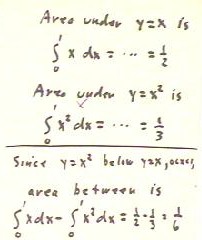
- We easily find that the area under the y = x curve is 1/2,
while that under the y = x ^ 2 curve is 1/3.
- The difference is clearly 1/6.
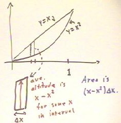
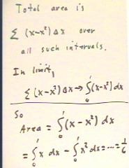
In the figure below we look at the idea behind the second strategy.
- For any small interval of the x axis, the corresponding region of the graph can be
approximated by a rectangle whose average altitude is x - x^2, where x is chosen somewhere
within the interval, and whose width is that of the interval, represented by the symbol
`dx in this example.
- The area of the small strip of the region is therefore approximately (x - x^2) * `dx.
The total area of the desired region is therefore the sum of the (x - x^2) * `dx
contributions, which is we know in the limit becomes the integral of x - x^2.
- It follows that the area is given by the integral indicated in the figure below.
- We note that this integral breaks up into the difference of the two area integrals used
with the first strategy.
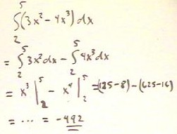
Below we show the details of integrating 3x^2 - 4x^3 the between x = 2 and x = 5.
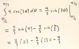
The antiderivative can be found by inspection, keeping the chain rule in mind, or by a
trial antiderivative of c sin(3 `theta).
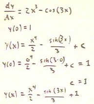
In the figure below we solve the differential equation dy / dx = 2x^3 - cos(3x) with
initial condition y(0) = 1.
- We first find the general antiderivative of the right-hand side, being sure to include
the arbitrary constant c so we can satisfy our initial condition.
- We then evaluate our antiderivative at x = 0 to determine the value of c.
- We easily determine that c = 1, and plug this value back into the general antiderivative
to get the particular antiderivative for the given initial condition.
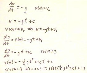
A freely falling object has acceleration -g, where g
is the magnitude of the acceleration of gravity.
- Since acceleration is the time derivative of velocity,
the above statement is translated as the differential equation dv / dt = -g.
- If we know the initial velocity v(0) = v0 of the object, we can solve
this differential equation for the function v(t).
- The solution is straightforward if we realize that the constant -g has
as an antiderivative - g t.
- We apply the initial condition to evaluate the constant c of
integration and obtain the velocity function v(t) = -g t + v0.
Now we note that the velocity of the object is the derivative
ds / dt of its position function.
- For the present case we conclude that the position function is
described by the differential equation ds / dt = v(t), or ds / dt
= - g t + v0.
- If we know an initial condition for the position function,
for example the condition s(0) = 1.3 of the example below, we can solve
the differential equation to obtain the position
function.
- We find an antiderivative of the right-hand side of
the differential equation, again including the integration
constant c.
- We then apply our initial condition to evaluate c,
obtaining the solution at the bottom of the figure below.
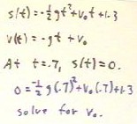
The final solution for the preceding problem is the function
s(t) given below.
- Note that the velocity function v(t) is indeed the derivative
of the position function.
- Suppose we know that the object strikes the ground at clock time t
= .7. Then, if we know the value of g we can set up an equation to
solve for v0.
- The equation is obtained by setting s(t) = 0 for t = .7.
- The resulting equation is given in the second-to-the-last line in
the figure below.
- If g is known, v0 is the only variable and we can easily
solve for v0.
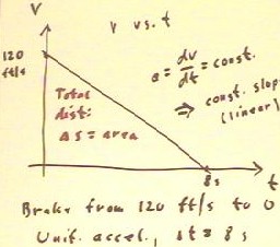
Consider now the problem of determining the total distance traveled by
an automobile which accelerates uniformly to v=0 in 8
s, starting with velocity of 120 feet/second.
- The total distance is the area under the velocity vs.
clock time graph.
Since the acceleration a = dv/dt = is constant, the slope
of the graph will be constant.
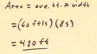
Is therefore easy to find the distance traveled by multiplying the average
velocity by the time interval.
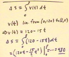
The area is easily found to be 480 ft, as indicated below.
The distance is also easily found as the integral
of the velocity function.
- The velocity function is a linear function from the
graph point (0, 120) to (8, 0).
- We easily find the linear function corresponding to these to graph points. The function
is v(t) = 120 - 15 t.
- Since velocity is the derivative of position,
change in position will be the definite integral of the velocity
function between the two clock times.
- We evaluate the integral at the bottom of the figure below.
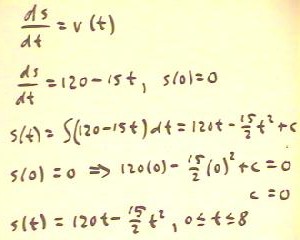
We can also solve the problem as a differential equation with an
initial condition.
- Since we are trying to relate position s and velocity v,
our differential equation will be ds / dt = v(t) = 120 - 15 t, as
indicated below.
- Since we are trying to find the distance traveled, we begin with
initial condition s(0) = 0, indicating that our starting distance is
zero.
- The position function is the general antiderivative of
120 - 15t, including the integration constant c as indicated below.
- The initial condition s(0) = 0 implies that c = 0.
- We therefore obtain the position function shown in the last
line of the figure below.
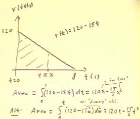
To obtain the distance function as an area integral,
we can find the position change from clock time t = 0 to
the variable clock time t = x.
- The position change is indicated by the area of the shaded
region of the graph below.
- This area is the integral from t = 0 to
t = x of the velocity function, as indicated below.
- If we complete the integration we find that the distance is s(x) = 120 x - 15/2
x^2.
Note that the symbol t disappeared when we substituted the limits of
our integral, and our clock time for the distance function is
now represented by x.
It doesn't make a lot of sense to use x for a clock time. We might be better off using
the integral in the last line below.
- In this integral we use t instead of x as our limit
of integration, and instead of using t as the variable
of integration we use a 'dummy variable' w.
- When we complete the integration we will have the area function 120 t - 15/2 t^2,
which is the same as the function obtained before except with t as
the variable.
- The use of w as the variable of integration makes no
difference, since we will be substituting t and 0 for the
variable, with the result that w doesn't appear anywhere in the solution.
We see that the distance function obtained in the previous
example is in fact an antiderivative of the velocity
function.
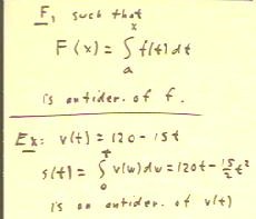
- In general, as indicated below, a function F such that F(x) is
the definite integral of f(t), between some fixed
limit a and the variable limit x, must be an antiderivative
of the function f.
- This result is known as the Second Fundamental Theorem of Calculus.
- As shown that the bottom of the figure below, the position function s(t) found
earlier is in fact an antiderivative of v(t).