integral approximation I

Calculus II

Class Notes, 2/03/99

We will compare the left, right, and trapezoidal approximations and actual integral of y = ln(x/2).

We first observe that since the function, whose graph is as shown below, is strictly increasing, the left approximation will be less than any of the others, the right approximation will be greater, and a trapezoidal approximation will lie between the left and right approximations.
We observe also that since the graph is concave downward, the region under the curve will always curve up and over the chord at the top of the trapezoid.

We conclude that the actual integral will always be greater than the trapezoidal approximation.

We therefore predict that the numerical results, listed in increasing order, will be left < trapezoidal < right < actual.

We proceed to calculate the values of the integral and of the n = 3 approximations for x = 2 to x = 11.

The same techniques will be used and the same ordering will be obtained for the original interval x = 2 to 20; you should complete these calculations.

We divide the interval from x = 2 to x = 11, whose length is 9, into 3 subintervals each of length 3.

The DERIVE vector command vector( [x, log(x/2) / log(2) ], x, 2, 11, 3) will give a table of y vs. x values. (Note error: in the figure, the x before the 2, 11, 3 is missing).

DERIVE could be used to calculate any of the approximations or the actual integral as follows:

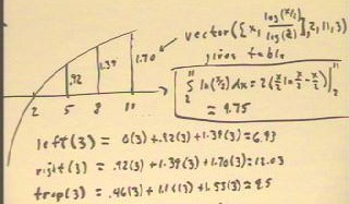
The DERIVE command vector ([log(x/2)], x, 2, 11, 3) will give a single-column listing of the values.

The DERIVE command sum (vector ([log(x/2)], x, 2, 11, 3) ) will give a sum of these values.

The DERIVE command 3 * sum (vector ([log(x/2)], x, 2, 8, 3) ) will give the left approximation.

The DERIVE command 3 * sum (vector ([log(x/2)], x, 5, 11, 3) ) will give the right approximation.

The DERIVE command 3 * sum (vector ([log(x/2) + log(x+3) / 2], x, 5, 8, 3) ) will give the trapezoidal approximation.

The DERIVE command 3 * sum (vector ([log(x/2)], x, 3.5, 9.5, 3) ) would give the midpoint approximation.

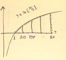
The DERIVE command int( log(x/3), x, 2, 11) would give the actual integral.

The graph below depicts the values of the function at x = 2, 5, 8 and 11.

The 'left' altitudes will occur at x = 2, 5, and 8, and each will be multiplied by the 3-unit width of the corresponding interval to get the left approximation. The results are shown in the figure.

The 'right' altitudes will occur at x = 5, 8 and 11, and the results are shown.

The 'averages' of left and right altitudes, used for the trapezoidal approximation, are .46, 1.16 and 1.55; each is multiplied by the width of its interval to obtain the trapezoidal approximation, as indicated.

The integral is easily calculated using either integration by parts or a table.

We see that, as expected, the left approximation is the smallest, the right the largest, and the trapezoidal approximation is less than the actual integral.

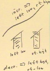
The figure below shows why when a function is increasing the left approximation is low and the right is high.

Similarly if the function is decreasing we conclude that the right approximation is low and the left high.

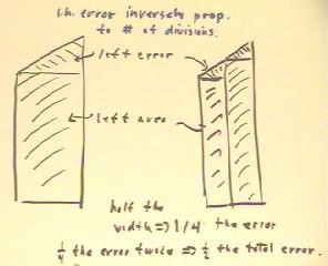
The figure below shows how the error of the left approximation changes as the width of the interval is halved.

Note that for sufficiently small intervals, each region under the graph will be an approximate trapezoid.

The left error for each trapezoid is the area of the triangle at the top of the trapezoid.

When the width of a trapezoid is halved, both the base and the height of the 'error triangle' are halved so that the left error becomes 1/4 as great.

When a trapezoid is subdivided into two trapezoids, then, each of the two trapezoids will have approximately 1/4 the error of the original so that the total error will be 2 * 1/4 as great, or 1/2 as great.

This argument makes it very plausible that the left-hand error of the approximation is inversely proportional to the number of divisions, to the extent that the number of divisions is large enough that each subregion is in approximate trapezoid.

A very similar argument where we subdivide each trapezoid into n subregions would prove this proportionality.

One result is that therefore if we use 10 times as many subdivisions, our error is reduced by a factor of 10 and we obtain an extra decimal place in the accuracy of our approximation.

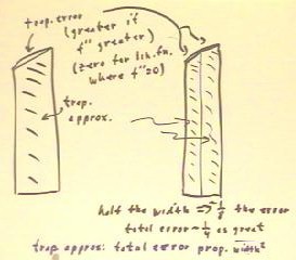
For a trapezoidal approximation, the error is the small 'crescent' between the top of the trapezoid and the actual curve.

The second derivative and the width of the interval determine how much the actual curve arcs above or below the trapezoid.

If the arced region above the trapezoid is regarded as an approximate triangle, then width of the interval and the difference between the actual slope at the left and the right end of the trapezoid determines the altitude of the triangle.

If the width of the trapezoid is halved, the difference in the slopes will be cut in half, and the difference will apply over only half the distance, so the altitude of the 'triangle' will be only 1/4 as great.

Since the 'triangle' will have only 1/4 the altitude and 1/2 the width its area will be only 1/8 as great.

Thus when a trapezoid is subdivided into two trapezoids, each of the two will have only 1/8 the error of the original and the total error of the two will be 2 * 1/8 = 1/4 as great as before.

1/4 is the square of 1/2, the proportion by which we reduced the width.

We therefore see the plausibility of the argument that the error of the trapezoidal approximation is inversely proportional to the square of the the number of divisions, or proportinal to the square of the width.

If the proportionality holds, then 10 times as many divisions would result in 1/10^2 = 1/100 the error and our accuracy would therefore improve by two decimal places.

Note that 10 times the number of divisions for the left approximation gave us just 10 times the accuracy, or 1 decimal place improvement, whereas the same change for a trapezoidal approximation gave us 100 times the accuracy and a 2 decimal place improvement.

We get 100 times the improvement for 10 times the work by using the trapezoidal approximation as opposed to the left approximation.