Next Time

Quiz 0330

1.  If we start with $1000 and compound interest at 8% annually, then

• What is our growth rate?
• What is our growth factor?
• How much money do we have after 10 years?
• How much money do we have after t years?
• During which year will our money first double?

The growth rate is .08, the growth factor is 1.08. 

After 10 years we have $1000 * 1.08^10 = 2158.92.

After t years we have

• P(t) = $1000 * 1.08^t.

After 10 years we have already doubled.  Checking 9 years we find that P(9) = 1999.00.  So just after the 9th year we will have doubled.

See further development of this topic at Properties of Exponential Functions below.

2.  In the preceding problem, suppose our amount after t years is $1000 * t^2.  Comparing this with the amount you get with the 8% annual interest:

• With which function would you have more money at the end of the first year?
• With which function would you have more money at the end of the second year?
• With which function would you have more money at the end of the tenth year?
• Do you think this function will be the best deal for the rest of your life?
• Do you think this function will be the best deal forever?
• Which function gives you the greater total for 100 years?
• Approximately how long does it take the first function to double? 
• How many doublings will take place in 100 years?
• If t = 10, then how long does it take t^2 to double?
• If t = 100, then how long does it take t^2 to double?
• Estimate the value of t at which the t^2 function will first take longer to double than the exponential function.
• Write an equation to determine the value of t at which the doubling time of the t^2 function first exceeds that of the exponential function.

If we use Q(t) = $1000 t^2 to stand for this function, which you should note is a power function, and P(t) = $1000 * 1.08^t for the exponential function we find the following:

• Q(1) = $1000 * 1^2 = $1000, while P(1) = $1000 * 1.08^1 = $1080.  So the power function is behind after 1 year.
• Q(2) = $1000 * 2^2 = $4000, while P(2) = $1000 * 1.08^2 = $1166 approx..  So the power function jumps way ahead after 2 years.
• Q(10) = $1000 * 10^2 = $100,000, while P(10) = $1000 * 1.08^10 = $2160, approx..  The power function has jumped way, way ahead.
• Q(100) = $1000 * 100^2 = $10,000,000, while P(100) = $1000 * 1.08^100 = $2,200,000 approx.  The power function is still way ahead, but it's now only about 5 times as great while it was about 50 times as great.
• Extending this to 200 years we find that Q(200) = $40,000,000.  However P(200) = $4,000,000,000 approx. about 100 times as great.  So the exponential has gone way past the power function.
• At t = 10 years the value of t^2 is 10^2 = 100.  To double to 200 we would need t^2 = 200, or t = sqrt(200) = 14.14 approx.   So it takes about 4.14 years for t^2 to double.
• The exponential function requires 9 years to double.  So at this point the t^2 function is doubling faster than the exponential function.
• At t = 100 years the value of t^2 is 100^2 = 10,000.  To double to 20,000 we would need t^2 = 20,000, or t = sqrt(20,000) = 141.4 approx.   So it takes about 41.4 years for t^2 to double at this point.
• The exponential function is still doubling every 9 years.  So the exponential function is at this point doubling in less than 1/4 the time of the power function.
• The slower and slower doubling of the power function, contrasted with the constant doubling time of the exponential, allows the exponential to catch up and blaze on past the power function somewhere between t = 100 and t = 200.

The idea of doubling time is further developed at doubling time below.

3.  The table below shows the temperature T of a soft drink as a function of clock time t in a room whose temperature was 25 C.

Let Tdiff by the difference between the temperature and room temperature.   For example, at clock time t = 0 we have Tdiff = 25 C - 5 C = 20 C.

Make a table for Tdiff vs. t and quickly sketch a graph of Tdiff vs. t.

Does the graph increase at a increasing rate, increase at a decreasing rate, decrease at an increasing rate or decrease at a decreasing rate?

Does the graph have an asymptote, and if so what is it?  Why should it be so?

The graph of Tdiff vs. t decreases at a decreasing rate.  It is asymptotic to the x axis, because the temperature of the soft drink approaches the temperature of the room as a limit, which means that the temperature difference approaches zero.

See the further development of this topic and the topic of question 4 below at Temperature vs. clock time data and analysis.

4.  Make a table of log(Tdiff) vs. log(t), and another table of log(Tdiff) vs. t. 

We get the table below:

Which table do you think would give you the more nearly linear graph?

It turns out that a carefully made graph gives us a very nearly linear graph for log(Tdiff) vs. t.

This is great because we can always find a decent equation from the graph of a linear function by estimating slope and y intercept.

See the further development of this topic and the topic of question 3 above at Temperature vs. clock time data and analysis.

The following questions will be developed during our next class and will be related to the above:

5.  Make a table of y = x^2 vs. x, for x = 0, 1, 2, 3.  The first column of a y vs. x table contains the x values, the second column contains the y values.   Quickly sketch a graph of this table.

Now make a table which simply switches the two columns.  However don't switch the labels of the columns.  The first column will still read x and the second will still read y.  On the same graph you used before, sketch a graph of this table.

How do the two graphs compare?

The second table represents a function, which is the function inverse to y = x^2.  What are the values on this table corresponding to x = 4 and x = 9?  What is your estimate of the value of this function for x = 6?

6.  Make a table of y = 10^x for x = -3, -2, -1, 0, 1, 2, 3.  Quickly sketch a graph.

Now make a table for the function which is inverse to this function.   Quickly sketch its graph.

How do the two graphs compare?

Does either graph contain an asymptote?  What are the asymptotes of these graphs, if any?

What is the value of the inverse function for x = .01?  What about x = 1000?

What do you estimate the value of the inverse function to be for x = 50?

#Precalculus I Class 03/11 includes temp model, linearizing

#Precalculus I Class 03/13  more linearizing, inverse functions

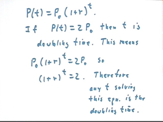
Doubling Time

We want to solve the equation 2P0 = P(t)

P(t) = P0(1 + r)^t

The doubling equation 2 P0 = P(t) becomes

• 2P0 = P0(1 + r)^t

If we divide both sides by P0 we get

• 2 = (1 + r)^t

How do we solve for t in the equation 2 = (1 + r)^t?

To solve the equation for t you need to use logarithms, which we haven't done yet (soon, within a couple of weeks).

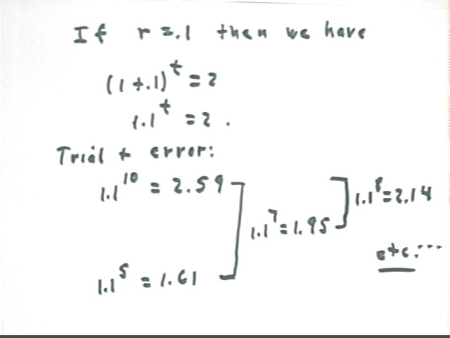
The only alternative is to solve by trial and error.  To do this you need a numerical value for r.

For example if r = .1 we have

• 2 = (1 + .1) ^ t or
• 2 = 1.1^t.

We first find a value for t that makes the result bigger than 2.  t = 10 is a good choice, giving us

• 1.1^10 = 2.593

Now we find a value that makes the result smaller than 2:

• 1.1^5 = 1.61.

Now we've got the number 2 'bracketed' between 1.1^5 = 1.61 and 1.1^10 = 2.59.

We now pick an exponent between 5 and 10.  To keep it simple we'll use either 7 or 8.  The class has chosen 7.  We find that

• 1.1^7 = 1.95.

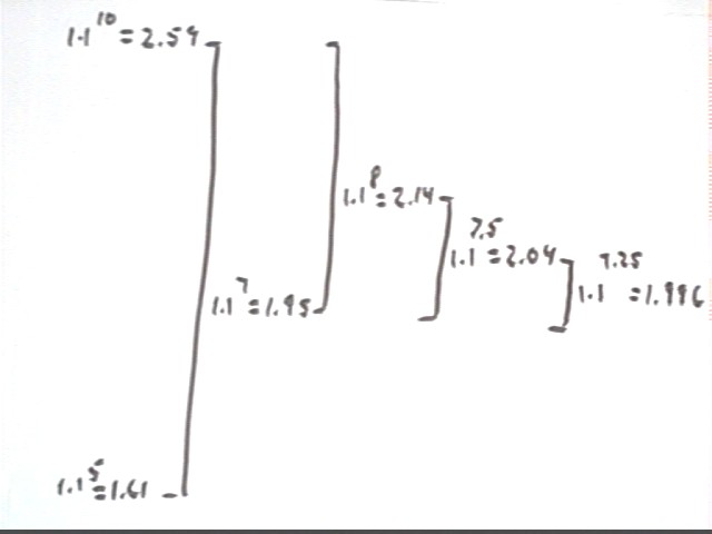
We have narrowed our bracket to the interval [7, 10].  We choose a number in this interval.  A quick look at the numbers tells us that 8 is a good choice.

• 1.1^8 = 2.14.

Now our bracket is [7, 8].  Taking the midpoint of our bracket we evaluate the number at 7.5:

• 1.1^7.5 = 2.04.

Now our bracket is [7, 7.5].  Taking the midpoint of our bracket we evaluate the number at 7.25:

• 1.1^7.25 = 1.996.

Now our bracket is [7.25, 7.5]. 

We could continue to refine our brackets but we're confident that the result to 2 significant figures is 7.3.

We can make this process as accurate as we like.

The bracketing process is illustrated below:

Quick preview of solution to 2 = (1 + r)^t:

Take log of both sides to get

• log(2) = log( (1+r) ^ t). 

Laws of exponents reversed for logs give us

• log(2) = t log(1+r) so that
• t = log(2) / log(1+r).

For example if r = .1 we have

• t = log(2) / log(1.1) = 7.2725.

Precalculus I Class 03/11

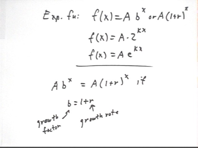
Properties of Exponential Functions

Recall that an exponential function is characterized by a growth factor and a growth rate.  If the growth rate is r then the growth factor is 1 + r and the function can be expressed as f(x) = A ( 1 + r)^x.

• f(x) = A ( 1 + r)^x can also be written as f(x) = A * b^x, with b = 1 + r.  In this form we call b = 1 + r the growth factor.

• Other forms we will encounter are f(x) = A * 2^(kx), which is obtained from the basic exponential function y = 2^x by vertically shifting it by factor A, then horizontally compressing it by factor k.

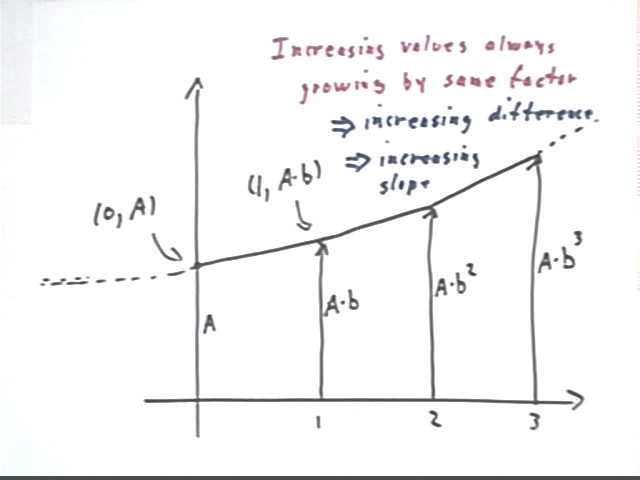
The graph of the exponential function y = A b^x has basic points (0, A) and (1, A * b).

The values of this function at x = 1, 2 and 3 are A b, A b^2 and A b^3.  Each time x changes by 1, the value of y increases by factor b (which you should recall is the growth factor).

• For example if the function represents the principle with annual compounding of interest, the value 1 year in the future will always be b times higher, no matter on which year you start. 

Applying the same positive growth factor at equal intervals, we apply the growth factor to increasing values.  It follows that the change in the amount (which is based on the original amount) will also be increasing.   This results in an increasing slope.

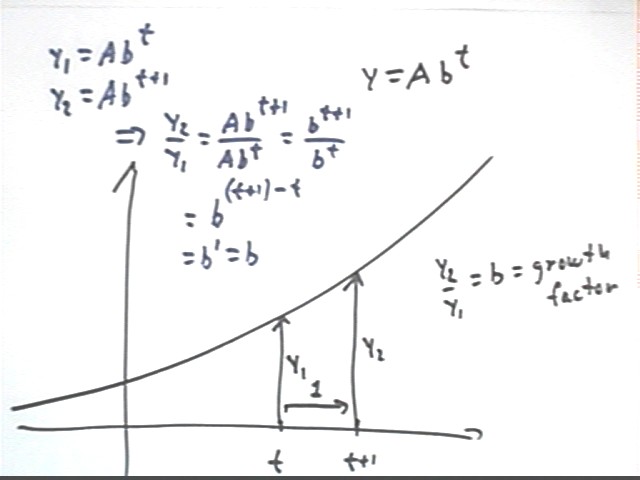
We algebraically prove that for the function y = A b^t, the amount 1 year later is always b times the current amount.  

• Let t be any time whatsoever.

• Then 1 year later the time will be 1 + t.

• If we let y1 and y2 be the amounts at times t and 1 + t, we find that 

y1 = A b^t and

y2 = A b^(t+1).

• Thus the ratio of the two values will be y2 / y1 = A b^(t+1) / A b^t.  This expression simplifies, as shown below, to just b.  This proves the result.

The following observations were made of the temperature reading on a thermometer vs. clock time t.  The thermometer was removed from a cold bottle of soft drink, dried and exposed to the air in the room, which was at temperature 25 C.

Is the temperature increasing at a constant, an increasing or a decreasing rate.

It's difficult to tell for sure from individual data points, which are a bit uncertain because the instructor who was reading the thermometer really needed to be using reading glasses but wasn't.  

However it isn't difficult to see from the temperatures, which were observed at regular intervals, that the tendency is for temperature differences to decrease so that the graph will be increasing at a decreasing rate.

Sketch and describe your graph of temperature vs. clock time, and confirm whether or not the temperature appears to be increasing at a decreasing rate.

A graph of temperature vs. clock time is depicted below.   It is clear that the temperatures tend to increase at a decreasing rate, since the tendency of the slope is to decrease as t increases.

Why do you think that the rate of increase is decreasing?

Most people present said that the closer we get to room temperature the less influence the room temperature has on the temperature of the thermometer.  This is an accurate perception.  

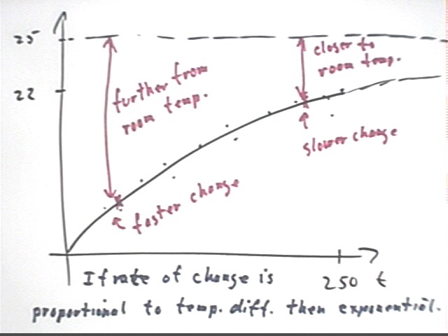
Physics can refine this perception and make it more precise.  It turns out that the influence of room temperature on the temperature of the thermometer is fairly complicated, but to a significant degree of accuracy the rate of temperature change is directly proportional to the difference between the temperature of the thermometer and that of the room.

In the figure below we indicate what this means:

• The dotted line at T = 25 indicates the room temperature Troom = 25 C.

• The exponential function representing temperature approaches Troom as its asymptote.

• When temperature difference is greater the temperature is seen to change at a greater rate.

An exponential function is characterized by the direct proportionality between the difference between the function value and the rate of change of that value. Exponential functions arise when this is the case, and every exponential function has this characteristic.

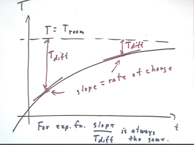
Making the above statements more precise we indicate Tdiff at two points, and the line segments indicating the slopes at those points.

• Where Tdiff is greater we see that the slope is greater.

• In fact if Tdiff is 3 times as great at one point as at another, the slope should also be 3 times greater at that point than at the other.

This direct proportionality can be indicated by the fact that slope / Tdiff is the same at all points.

• Note that this is a direct proportionality, not a proportionality of the square or cube or anything else (i.e., slope / Tdiff is constant, NOT for example (slope / Tdiff)^2 or (slope / Tdiff)^3) ) .  It's a proportionality of the first power.

Excel isn't too smart.  DERIVE is smarter than Excel but still not smart enough.  The curve-fitting algorithm in Excel can only fit an exponential accurately if the asymptote is the x axis.  It just can't handle an asymptote at, say, T = 25.

However if we know the asymptote we can trick Excel into giving us what we need.

We note that as temperature approaches its asymptotic value the temperature difference 25 - T shrinks.  The temperature difference therefore approaches zero as an asymptote, and Excel can handle this type of data.

• The table below is identical to the table given previously except that we have included a column for Tdiff.

• We have included a graph of Tdiff vs. t, indicating the Excel exponential fit 

Tdiff = 2-.5 e^-.0073 t.

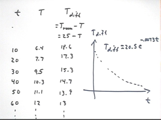
The table below shows all the observed values of Tdiff:

The graph below shows T vs. t as before, with T approaching 25, but also shows Tdiff as the decreasing exponential function with asymptote 0.

The graph of the best-fit exponential function is depicted as is the function itself.  The function uses y and x to indicate the variables Tdiff and t.

There is another way to 'trick' computer algebra programs such as DERIVE into doing an exponential fit, which is something DERIVE is not designed to do.

The table below shows log(Tdiff) vs. t.  You can verify these values using your calculator and the log key.  Calculate the log of the first value Tdiff = 20 and you'll find that you get 1.30 approx., as shown in the table below.

If your data is exponential with asymptote zero then a graph of log(Tdiff) vs. t will result in a nearly straight line.

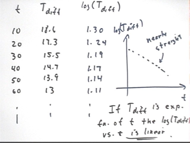
The table below shows all the Tdiff values for the data we collected.

The graph below shows log(Tdiff) vs. t, along with the best-fit straight-line approximation to this data.

• The straight line has equation y = -.0032 x + 1.312.  Since y represents log(Tdiff) and x respresents t, this equation could be represented as

log(Tdiff) = -.0032 t + 1.312.

This equation can be solved for Tdiff in terms of t.  However the equation involves logarithms, and to solve it will require that we first understand the properties of logarithms.

The solution of this equation, or any equation of this form with the log of one quantity being linearly dependent on another quantity, is an exponential function.

Observe that the data do not give us a perfectly straight line, with values first dipping below, then above, and finally once more below the straight line.

• The reasons for the most of the anomalies are quite complex, requiring the application of much higher-level mathematics to the physics of the situation.
• Some of the anomalies, especially near the end of the graph, are likely the result of an error in estimating the room temperature, which was in fact not observed very carefully.

The graph shown below results if we use T = 26 for the room temperature.

• Note that while this graph still has the same type of behavior as the preceding, it is significantly closer to the straight line, especially at the right-hand end of the line segment but also at other points.
• We conclude that room temperature might indeed have been closer to T = 26 C than to T = 25 C.

Room temperature T = 27 C gives us an even better fit.  However it is unlikely that the temperature was really this high.

Room temperature of T = 28 C and T = 29 C give us the graphs shown below.

Note that while the models appear better these temperatures are definitely higher than those in the room.  The 'flattening' of the graph is due to other properties of exponential and linear functions.

Precalculus I Class 03/13

During the preceding class we linearized temperature vs. clock time data by using a log(T) vs. t transformation. 

Here we will illustrate the general process we will use in this course to linearize data. 

The y vs. x table shown below is built using the y = 5 x^3 function.  Usually when we linearize data we don't know what the best function is (as was the case with the temperature data), but for this illustration we'll start with a known function.

• Our first step is to create log(x) and log(y) tables, which is easily done using calculator or spreadsheet.

• We will then create graphs of log(y) vs. log(x) and log(y) vs. x.  A third type of graph we might sometimes use is y vs. log(x), though for this illustration we'll stick to the first two.  

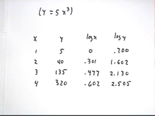
A more accurate table is shown here:

 Our graphs will be set up as illustrated below.

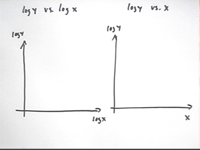
Graph of log(y) vs. x is not very linear, increasing at a decreasing rate:

The graph of log y vs. log x is pretty much linear, increasing at what appears to be a constant rate.

The straight line through these data points has an equation of form log(y) = m * log(x) + b, where m is slope and b is the vertical intercept.

• The specific function that fits our graph has slope 3 and vertical intercept .699.  

• The best-fit function might not be given by your software in appropriate form.  Excel, for example, will tell you that the resulting function is y = 3 x + .699.  However we know that the graph is not y vs. x but log(y) vs. log(x) so we write this function as log(y) = 3 log(x) + .699.

• In the graph below we have changed Excel's y = 3 x + .699 to the more appropriate log y = 3 log x + .699.

Our results correlate with the power function we used to generate the data.  We haven't yet developed the tools to see precisely how these relationships exist.  However for future reference:

• We note that the slope 3 matches the power of the power function y = 5 x^3 we used to generate the data.

• Also check out the fact that 10^.699 = 5, which matches the coefficient of our power function.

For reasons that we'll see later, a power function y = A x^p will result in a log y vs. log x graph whose slope is p and whose y-intercept b has the property that 10^b = A.

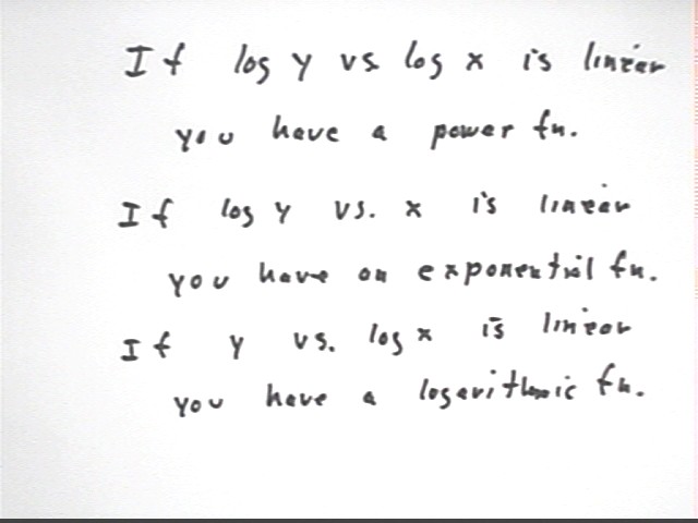
We will see in upcoming classes why the following general rules for linearization hold:

We now investigate the idea of inverse functions.

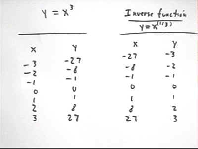
• We start with a table for y = x^3.

• To get a table for the inverse function we reverse the numbers in the two columns.

Our original function is y = x^3.  We obtain the formula for the inverse function as follows:

• We first reverse the roles of x and y in the formula y = x^3, obtaining x = y^3.

• We then solve the reversed equation for y.  We do this as follows:

x = y^3.  We take the 1/3 power of both sides, obtaining

x^(1/3) = (y^3)^(1/3).  We use laws of exponents to simplify the right-hand side and get

x^(1/3) = y.  We switch the two sides to obtain

y = x^(1/3).

We sketch a graph of the function and the inverse function and note its significant characteristics:

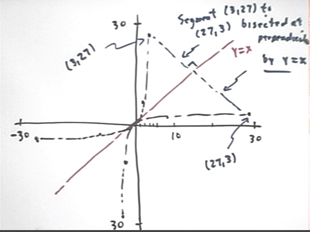
• The graph of the inverse function is obtained by reversing the coordinates of the points on the graph of the original function.

• The result is that every point on the graph of the original function can be joined to the corresponding point on the graph of the inverse function by a line segment which (provided the graph is drawn with equal scales for the x and y axes) is perpendicular to the line y = x and which is bisected by this line.

• For example, (3, 27) on the graph of y = x^3 corresponds to the point (27, 3) on the graph of the inverse function y = x^(1/3).  If we join (3, 27) to (27, 3) by a line segment that segment passes through the graph of y = x at a right angle.  This segment is bisected (i.e., cut into two equal parts) by the y = x graph.

The main characteristic of a graph of a function and its inverse is that the two functions are symmetric with respect to reflection about the line y = x.

An accurate plot of these functions is shown below:

'Zooming in' on the domain 0 <= x <= 3:

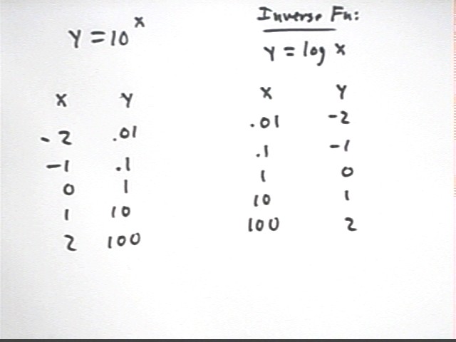
The log function y = log(x) is defined as the inverse of the y = 10^x function.

• Note that if we switch coordinates in the expression y = 10^x we get x = 10^y.  The equation y = log(x) is therefore equivalent to the equation x = 10^y.

A table of y = 10^x and the 'inverted' table y = log(x) is shown below.

A rough graph of these functions is depicted below.   The graph in the lower-left-hand corner is an enlarged graph of these functions near the origin.

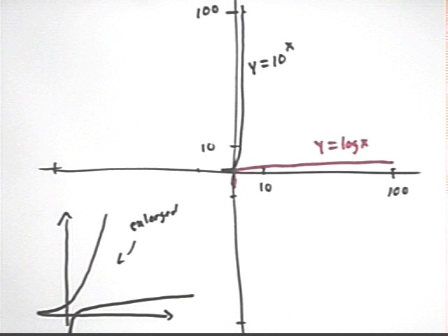
The figure below is a more accurate graph showing y = 10^x, y = log(x) and y = x.  Note the symmetry of these graphs with respect to reflection thru the line y = x.

A closeup of the same graphs near the origin shows the following important characteristics:

• The graph of y = 10^x passes through (0, 1), is asymptotic to the negative x axis and increases at an increasing rate.

• The graph of y = log(x) passes through (1, 0), is asymptotic to the negative y axis and increases at a decreasing rate.

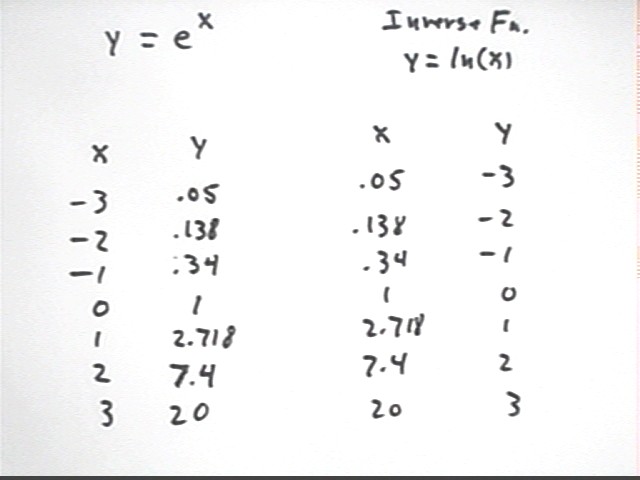
A closeup of the same graphs near the origin shows the following important characteristics:

• The graph of y = e^x passes through (0, 1), is asymptotic to the negative x axis and increases at an increasing rate.

• The graph of y = ln(x) passes through (1, 0), is asymptotic to the negative y axis and increases at a decreasing rate.

A comparison between the graphs of y = 10^x and y = log(x), and the graphs of y = e^x and y = ln(x), reveals the following:

• The x and y intercepts (0, 1) and (1, 0) are the same for the pair y = 10^x and y = log(x), and for the pair y = e^x and y = ln(x).

• The graphs of y = e^x and y = ln(x) change more gradually than those of y = 10^x and y = log(x), approaching their asymptotes more slowly and changing curvature more gradually.