Quiz 0422
4. On a graph that runs from x = -4 to x = 4, with y values running from -10 to 10, sketch a graph of two straight lines each with slope 1, one having x intercept -2 and one with x intercept +1.
The graph looks like this:
The y coordinates are -1 and -4, easily reasoned out. The sum is -5.
The sum graph would contain the point (-3, -5).
The y coordinates are +1 and -2, giving us a sum of -1.
The sum graph would contain the point (-1, -1).
The y coordinates are +4 and +1, giving us sum 5 and point (2, 5).
The y coordinates are +3 and +6, giving us sum 9 and point (4, 9).
Plotting the points and connecting with a straight line we get the new straight line in the figure below, having slope 2.
The sum of the y coordinates at x = -3, -1, 2 and 4 are -5, -1, 5 and 9.
The y coordinates of the first graph at these points are -1, 1, 4 and 6.
The sum of the y coordinates isn't the same as the y coordinate of the first line at any of these points.
The sum of the y coordinates will be the same as the y coordinate of the first line when the y coordinate of the second line is 0. That is, you get the same thing when you add zero.
The y coordinate of the second line is zero at x = 1, so at x = 1 the sum of the y coordinates will be the same as the y coordinate of the second line. Thus, the first line and the sum graph cross at the x = 1 point of the first graph.
The graph below includes the vertical line at x = 1 and illustrates how first line and the sum graph cross at the x = 1 point of the first graph, where the y coordinate of the first graph is 0.
Using the same reasoning as before, this will occur where the y coordinate of the first graph is zero.
The graph below includes the vertical line at x = -2 and illustrates how first line and the sum graph cross at the x = -2 point of the second graph, where the y coordinate of the second graph is 0.
5. Again sketch the two straight lines described in #4.
The y coordinates are -1 and -4, easily reasoned out. The product is +4.
The product graph would contain the point (-3, 4).
The y coordinates are +1 and -2, giving us a product of -2.
The product graph would contain the point (-1, -2).
The y coordinates are +4 and +1, giving us product +4 and point (2, 4).
The y coordinates are +3 and +6, giving us product 18 and point (4, 18).
If we plot the points we have obtained and sketch a smooth curve through the points we get something that looks very much like a parabola, as shown below.
The two graphs represent linear functions. When we multiply two linear functions we get a quadratic function.
Whenever we find the product of two straight-line graphs we will get a parabola.
This occurs when the y coordinate of the first line is 1. You get the same number when you multiply a number by 1.
The y coordinate of the first line is 1 when x = 2, so at x = 2 the product will be equal to the y coordinate of the second graph. We have actually evaluated the product at this point, obtaining the point (2, 4).
We can see that the graph of the product function crosses the graph of the first function at (2, 4).
The figure below includes the horizontal line y = 1 and the vertical line x = 2. These lines intersect at the graph of the second straight line. Be sure you understand why the vertical line x = 2 must therefore intersect the graph of the parabola.
This occurs when the y coordinate of the second line is 1. You get the same number when you multiply a number by 1.
The y coordinate of the second line is 1 when x = -1, so at x = -1 the product will be equal to the y coordinate of the first graph. We have actually evaluated the product at this point, obtaining the point (-1, -2).
We can see that the graph of the product function crosses the graph of the first function at (-1, -2).
The figure below includes the horizontal line y = 1 and the vertical line x = -1. These lines intersect at the graph of the first straight line. Be sure you understand why the vertical line therefore x = -1 must intersect the graph of the parabola.
This occurs when either of the y coordinates is zero.
The y coordinate of the first graph is zero when x = -2, so the product function will be 0 when x = -2 and the point (-2, 0) will occur on the graph of the product function. It is clear from the above graphs that the parabola does pass through this point. At this point the parabola intersects the first straight line.
Similarly the product function will be 0 at x = 1, when the second function is zero, and the graph of the product function will therefore intersect the graph of the second straight line at the point (1, 0).
At x = 1.5 the y coordinate of the second graph is .5. When we multiply the y coordinate of the first graph by 5 the result will be smaller in magnitude than that coordinate (this is because the magnitude of .5 is less than 1, and multiplying a number by another number of magnitude less than 1 decreases its magnitude).
This means that the x = 1.5 point of the product graph will be closer to the x axis than the first graph.
The figure below shows this behavior. The vertical line x = 1.5 intersects the graph of the second linear function on the line y = .5, showing that the second function has y value .5 at x = 1.5. The y value of the first function at this point is easily determined by following the x = 1.5 line up to the graph of the first function then across to the y axis. We see that the first function intersects the x = 1.5 line on the y = 3.5 line, so the first function has value 3.5.
When we multiply this value by the value .5 of the second function we get half the value (in this case y = .5 * 3.5 = 1.75). This is easily seen on the graph, where the parabola representing the product function meets the x = 1.5 line halfway between the y = 3.5 point of the first graph and the x axis (i.e., at x = 1.5 the parabola is exactly half as high as the first linear graph).
At x = .5 the y coordinate of the second graph is -.5. When we multiply the y coordinate of the first graph by -.5 the result will be smaller in magnitude than that coordinate (this is because the magnitude of -.5 is less than 1, and multiply a number by another number of magnitude less than 1 decreases its magnitude).
This means that the x = .5 point of the product graph will be closer to the x axis than the first graph, in fact twice as close.
Because of the negative in -.5 the product also 'flips' the result to the other side of the x axis.
The graph below shows how the line x = .5 intersects the second graph at y = -.5, and how the parabola intersects the x = .5 line twice as close to the x axis as to the first graph but on the other side of the axis.
The graph below shows the two linear functions and the parabola which is their product. The green and red lines represent y = 1 and y = -1. The second function lies between these lines between x = 0 and x = 2.
So for 0 < x < 2 the magnitude of the second function is less than 1, so the magnitude of the product is less than the value of the second function. At x = 0 the second function takes value -1, and we see that the product function (the parabola) is the same distance from the x axis as the first function but on the other side, which is what we expect from multiplication by -1. At x = 2 the second function takes value 1, and we see that for x = 2 the value of the first function and the product function are the same (the parabola intersects the first line at the x = 2 point).
Between x = 0 and x = 2, where again the magnitude of the second function is less than 1, it should therefore be clear that the product function is at every point closer to the x axis than the first function.
For reasons similar to those explained above, the y coordinate of the product will be closer to the x axis than the y coordinate of the second line whenever the magnitude of the y coordinate of the first line is less than 1--i.e., whenever the first line lies between the lines y = -1 and y = 1.
The figure below includes the vertical lines x = -3 and x = -1, between which the graph of the first linear function lies between y = -1 and y = 1. The product graph is closer at every point between x = -3 and x = -1 than the graph of the second linear function.
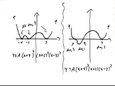
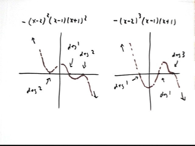
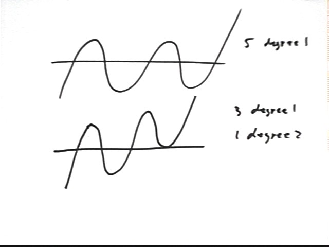
The graphs below both represent a polynomial of degree six with exactly three x value at which we get y = 0.
In the first all zeros are of degree 2, so the graph is very nearly parabolic near these points.
In the second one zero is of degree 3, resulting in a graph that levels off for an instant just as it passes thru the x axis. Another is of degree 1, passing through the x axis in a line which near the zero is very nearly straight, and the other is degree 2, giving us a near-parabola near the zero.
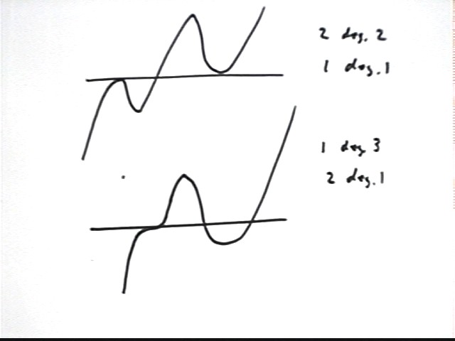
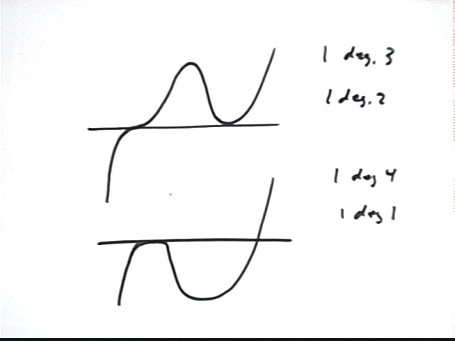
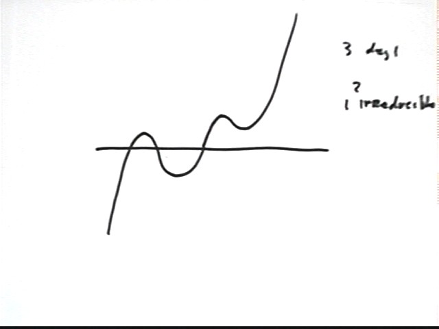
The three graphs below all have exactly three x-intercepts, as in the examples above.
All three also appear to be of even degree, since for large positive as well as large negative x they appear to approach +infinity.
In the graph immediately below the zeros appear to have degrees 1, 1 and 2, indicating a total degree of at least 4.
The next graph appears to have three zeros of degree 2, giving it total degree at least 6.
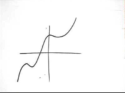
This graph appears to have zeros of degree at least 3, 1 and 2, for total degree at least 6.
The graph below could represent y = A(x+4)(x+2)(x-3)^2, with its first-degree zeros at x = -4 and x = -2 and its second-degree zero at x = 3.
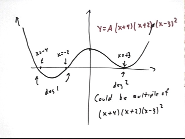
A more accurate graph of this function:
This graph could also conceivably represent y = A(x+4)(x+2)(x-3)^2 * (x^2 + x + 7), because (x^2+x+7) is an arbitrary irreducible quadratic (one we just picked out of a hat containing all irreducible quadratics).
x^2 + x + 7 is an irreducible quadratic because it has no zeros.
If we set x^2 + x + 7 = 0 and try to solve using the quadratic formula our solution will include sqrt(b^2 - 4 a c) = sqrt(1^2 - 4 * 1 * 7) = sqrt(-27), showing that there are no real values of x for which the expression is zero.
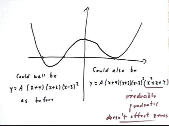
The irreducible quadratic x^2 + x + 7 has vertex at x = -b / (2a) = -1/2. The vertex is its 'low point' so it tends to 'depress' values more near x = -1/2 than away from that point. This causes a little less symmetry in the curve, as opposed to the preceding graph. Note how the curve between x = -2 and x = 3 appears to be a bit more lopsided than in the preceding graph.
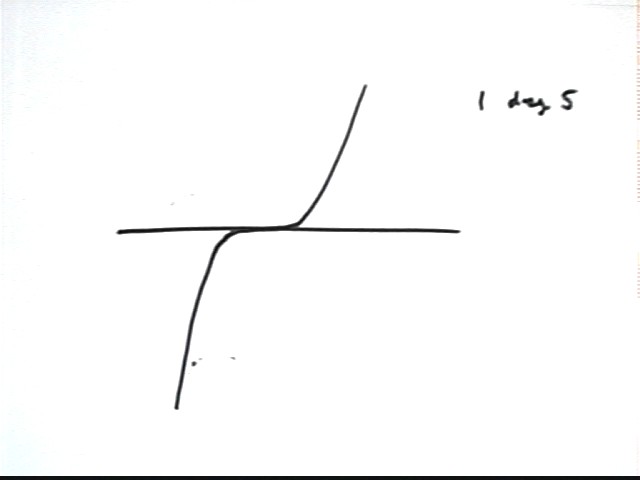
Suppose we know that a polynomial has degree 5. What is the maximum number of zeros it could have?
An example of a polynomial of degree 5 might be (x-3)(x-2)(x-1)(x+1)(x+2). This polynomial has 5 zeros, all different. We say that the polynomial has 5 distinct zeros.
If everyone in the class made up their own degree-5 polynomial with no zeros in common with the given polynomial it's very likely that they would all be different.
Suppose we know that a polynomial has degree 5. In how many different ways can we have, say, exactly 3 different numbers that give us zeros?
One possibility would be something like (x-2)^2 (x-1) (x+1)^2, with two of the zeros having degree 2. This polynomial actually has five zeros, since it can be written (x-2)(x-2)(x-1)(x+1)(x+1), but the zeros x = 2 and x = -1 are repeated zeros, each being repeated twice. Thus there are only three different numbers that give us zero, even though there are five zeros.
Another possibility might be of the form (x-2)^3 (x-1)(x+1), with one zero of degree 3 and the other two of degree 1.
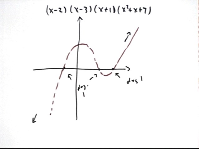
There is one more way we can get a degree-5 polynomial with exactly three different numbers that give us zero. That is to use an irreducible quadratic, as in the example (x-2)(x-3)(x+1)(x^2 + x + 7).
If the zeros are at -2, -1 and 1 then the following are examples of different ways to get polynomials of degree five with exactly three different x values for which the polynomial is zero:
(x-2)^2 (x-1) (x+1)^2
(x-2)^3 (x-1)(x+1)
(x-2)(x-3)(x+1)(x^2 + x + 7)
How can we have a degree 5 polynomial with exactly 4 numbers that give us zero? Sketch such a graph.
We can repeat one of the five zeros, for example getting (x-3)(x-2)^2(x-1)(x+1).
Precalculus I Class 04/10
For a degree-5 polynomial we can have any of the following:
We aren't done yet. We do have a list of every possible combination of five linear factors. However we haven't yet considered what happens if we have an irreducible quadratic (or two).
If there is one irreducible quadratic then we can have
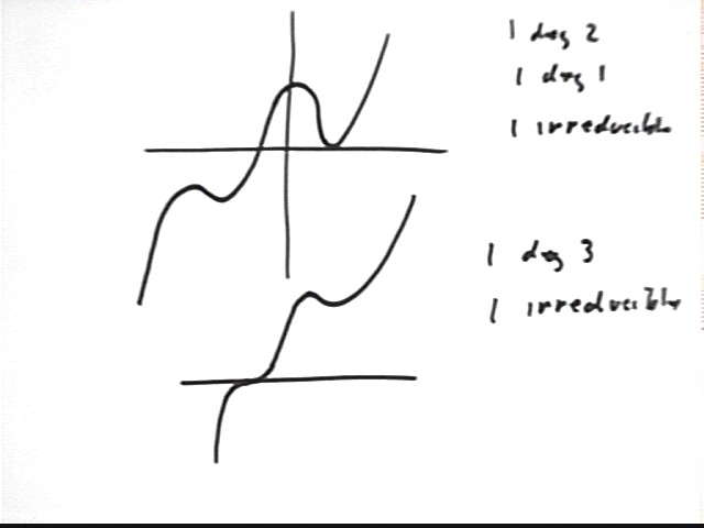
We can also have two irreducible quadratics. If so we must have one first-degree zero:
Evaluate e^x at x = .01, .1 and .2.
Evaluate 1 + x at x = .01, .1 and .2.
Evaluate 1 + x + x^2 / 2 at x = .01, .1 and .2.
e^.01 = 1.01005
1+.01 = 1.01. Note that this 'misses' e^.01 by .00005.
1+.01+.01^2 = 1.01010. This 'misses' e^.01 by .00005.
e^.1 = 1.10517
1+.1 = 1.1 'misses' e^.1 by about .005
1+.1+.1^2/2 = 1.105 'misses' e^.1 by about .00017
e^.2 =1.22140
1 + .2 = 1.2 'misses' e^.2 by about .021
1 + .2 + .2^2/ 2 = 1.22 'misses' e^.2 by about .001