Precalculus I Class 03/06
If we start with principle P0 and compound interest at an annual rate of 100%, compounding once annually, how much do we end up with at the end of a year?
What if we compound twice annually?
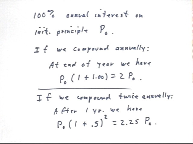
As shown in the figure below:
If we compound 100% annually, starting with P0, we end up at the end of the year with
(1 + 1.00) * P0 = 2 P0.
If we compound 100% twice annually, starting with P0, we apply 1/2 the 100% twice and end up at the end of the year with
(1 + 1.00/2)^2 * P0 = 2.25 P0.
Answer the same questions assuming that we compound 4 times annually (i.e., quarterly), monthly, weekly and daily? What if we compound 1000 times a year? What if we compound n times per year?
If we compound 100% four times annually, starting with P0, we apply 1/4 the 100% four times and end up at the end of the year with
(1 + 1.00/4)^4 * P0 = 2.44 P0.
If we compound 100% monthly, which is twelve times annually, starting with P0, we apply 1/12 the 100% twelve times and end up at the end of the year with
(1 + 1.00/12)^12 * P0 = 2.61 P0.
If we compound 100% weekly, which is 52 times annually, starting with P0, we apply 1/52 the 100% a total of 52 times and end up at the end of the year with
(1 + 1.00/52)^52 * P0 = 2.693 P0.
If we compound 100% daily, which is 365 times annually, starting with P0, we apply 1/365 the 100% a total of 365 times and end up at the end of the year with
(1 + 1.00/365)^365 * P0 = 2.71456 P0.
We see that the amount continues growing, but with each additional year the amount increases by less than in the preceding year.
If we compound 1000 times we end up with (1+1.00/1000)^1000 = 2.716923 P0 approx.
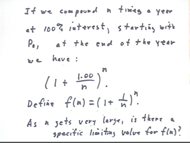
If we compound n times we end up with
end-of-year amount for n compoundings: (1+1.00/n)^n * P0.
Note that we report as many significant figures as we need to at least see the change from one number to the next. For n = 997 to n = 1004 the results (1 + 1/n)^n are shown below, and are seen to change in the 6th decimal place:
| number n of compoundings | (1 + 1/n)^n |
| 997 | 2.71691985 |
| 998 | 2.716921213 |
| 999 | 2.716922574 |
| 1000 | 2.716923932 |
| 1001 | 2.716925288 |
| 1002 | 2.71692664 |
| 1003 | 2.71692799 |
| 1004 | 2.716929337 |
Let f(n) = (1 + 1/n)^n. We've seen that
f(1) = 2
f(2) = 2.25
f(4) = 2.44
f(12) = 2.61
f(52) = 2.693
f(1000) = 2.716923
Using calculators we get
f(10,000) = 2.718145927
f(100,000) = 2.718268237
f(1,000,000) = 2.718281303 (note that many calculators will not give this result, due to the limitations of their arithmetic).
These numbers to approach a limit, which to 20 significant figures is
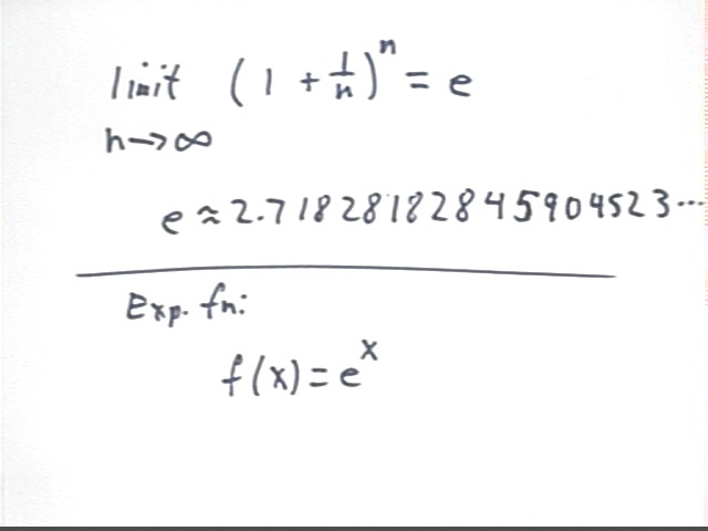
limit of (1+1/n)^n as n -> infinity is approximately 2.7182818284590452353.
This limit is an irrational number, never repeating, never establishing a pattern. We call the number e.
To 20 significant figures e = 2.7182818284590452353.
You should know that e = 2.718 approx.
Your calculator has an e^x button. If you calculate e^1 you will get the same result, up to the limit of your calculator's arithmetic.
The function y = e^x is the most basic of the exponential functions. We have also used y = 2^x as a basic exponential function. Your worksheets detail the relationship between these two functions.
Basically y = 2^x is the same as y = e^(kx) with k = ln(2). You will understand what this means in about a week.
Which grows faster, y = e^x or y = x^2?
We first study this question graphically. The figure below depicts y = e^x and y = x^2. At this point in the course you should know right away which is which.
We make the following observations:
y = e^x is clearly greater than y = x^2 for all positive values of x shown.
However for most positive values of x the graph of y = x^2 appears to be steeper than that of y = e^x, which would imply that y = x^2 might very well 'catch up with' and even surpass y = e^x.
On the other hand it might be that y = e^x is steepening more rapidly by the time we 'exit' the top of the page and that it will manage to stay ahead of y = x^2.
Before going on you should decide, based on what you see here, which function you think will 'win' in the long run.
In the figure below we 'zoom out' a bit. This picture shows us that the graph of y = e^x will in fact become steeper than that of y = x^2. The two graphs are parallel somewhere in the vicinity of y = 4, after which the y = e^x function becomes steeper.
Provided this pattern continues, the y = e^x function will get steeper faster than the y = x^2 function and will always stay ahead.
We now ask the same question of the y = e^x and y = x^3 functions. The figure below shows the two graphs near the origin. It is clear that the y = x^3 function is getting steeper more rapidly than the y = e^x function and it appears to be headed to 'victory'.
In fact the y = x^3 function does catch up to the y = e^x function around the point (1.8, 6).
The y = x^3 function continues steepen faster than the y = e^x function and it very much appears that this pattern will continue.
However zooming out once more (and note that the x and y scales are no longer equal as they were in the preceding graphs) we see that the steepness appears to again equalize by the time we reach y values around 40.
As we move further out we see that the y = e^x graph does indeed get steeper than the y = x^3 graph, and that the graphs again begin to grow closer.
Before we reach y = 100 the e^x graph is again ahead. You can verify that it will stay that way.
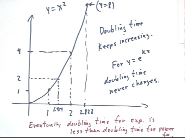
The reason that the y = e^x graph wins is that it doubles at regular intervals, while y = x^2 and other power functions require longer and longer intervals to double.
You should verify for yourself that y = e^x doubles every time x changes by .7.
You should also verify the doubling times depicted for y = x^2 in the graph below.
Starting at y = 1, which occurs for x = 1, we see that we reach y = 2 when x^2 = 2 or x = sqrt(2) = 1.414 approx.. So the y = x^2 graph doubles between x = 1 and x = 1.414, a 'doubling time' of .414.
The next doubling occurs as y increases from 2 to 4, which occurs between x = sqrt(2) = 1.414 approx. and x = 2. This doubling required a change in x of 2 - 1.414 = .584, greater than the previous 'doubling time'.
You should verify that the next doubling takes place between x = 2 and x = 2.828 approx., for an even greater 'doubling time' of about .828. Note that this 'doubling time' is greater than the doubling time of the exponential (which we saw was around .7).
Subsequent doubling times will follow this pattern, getting longer and longer.
Since the doubling time of the y = x^2 function eventually exceeds that of the y = e^x function it should be clear that the y = e^x function will eventually 'win'.
The same is true of the y = x^3 function. It takes longer for the y = e^x function to 'win' but it must eventually do so.
This pattern will continue for higher and higher powers of x. y = e^x always beats y = x^n eventually.
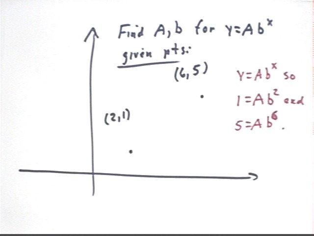
Problem: Find a and b such that y = A b^x for the points (2,1) and (6,5).
y = A b^x is a form for the exponential function, into which we may 'plug' any related x and y values.
We plug in the x and y coordinates to obtain the equations
1 = A b^2 and
5 = A b^6.
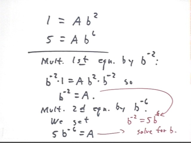
We can solve these equations using a variety of different strategies.
In the figure below we begin by solving the first equation for A, multiplying both sides by b^-2. We obtain
A = b^-2.
We could plug b^-2 in for A in the second equation, obtaining 5 = b^-2*b^6 or 5 = b^4, which we could easily solve for b. However that's not what we do below. Instead we solve the second equation for A:
Solving the second equation for A we multiply both sides by b^-6, obtaining A = 5 b^-6.
We then observe that we have two expressions for A, A = b^-2 and A = 5 b^-6.
These two expressions for A must be equal. So we obtain the equation
b^-2 = 5 b^-6.
We easily solve this for b, first multiplying both sides by b^6 to get
b^4 = 5
then finding the 1/4 power of both sides to get
b = 5^(1/4).
We would plug b = 5^(1/4) = 1.495 approx. into either of the original equations and solve that equation for A.
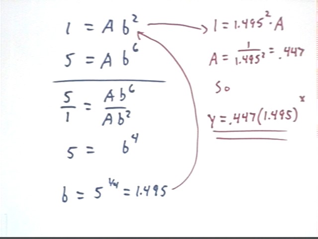
Another alternative solution to the system
1 = A b^2
5 = A b^6
is obtained by dividing one equation by the other, which will eliminate A.
Dividing the second equation by the first we end up with
5/1 = (A b^6) / (A b^2)
which we simplify to get
5 = b^4.
This gets us to the same point we reached in the previous solutions. We again find that b = 5^(1/4) = 1.495 approx.
Plugging this back into the first equation (follow the red arrows) we obtain
1 = A * 1.495^2,
which we easily solve to obtain A = .447.
It follows that our exponential function y = A b^x is
exponential function containing points (2,1) and (6,5) is
y = .447 * 1.495^x,
which is accurate to 3 significant figures.