Precalculus I Class 03/11
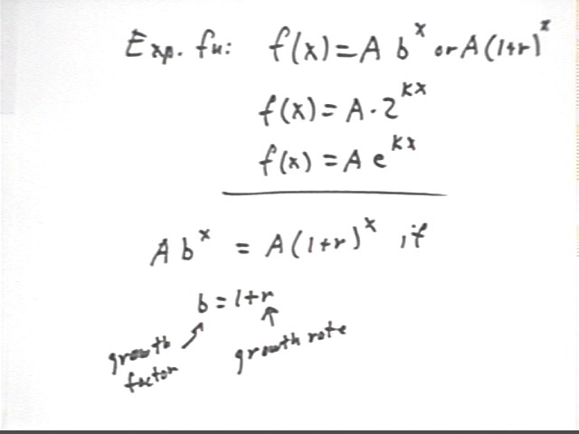
Recall that an exponential function is characterized by a growth factor and a growth rate. If the growth rate is r then the growth factor is 1 + r and the function can be expressed as f(x) = A ( 1 + r)^x.
f(x) = A ( 1 + r)^x can also be written as f(x) = A * b^x, with b = 1 + r. In this form we call b = 1 + r the growth factor.
Other forms we will encounter are f(x) = A * 2^(kx), which is obtained from the basic exponential function y = 2^x by vertically shifting it by factor A, then horizontally compressing it by factor k.
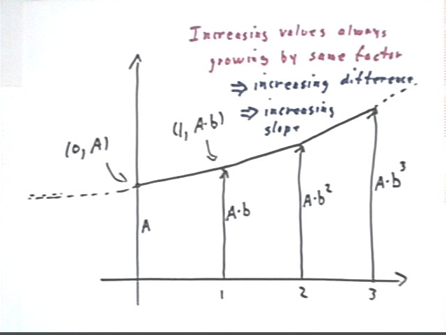
The graph of the exponential function y = A b^x has basic points (0, A) and (1, A * b).
The values of this function at x = 1, 2 and 3 are A b, A b^2 and A b^3. Each time x changes by 1, the value of y increases by factor b (which you should recall is the growth factor).
For example if the function represents the principle with annual compounding of interest, the value 1 year in the future will always be b times higher, no matter on which year you start.
Applying the same positive growth factor at equal intervals, we apply the growth factor to increasing values. It follows that the change in the amount (which is based on the original amount) will also be increasing. This results in an increasing slope.
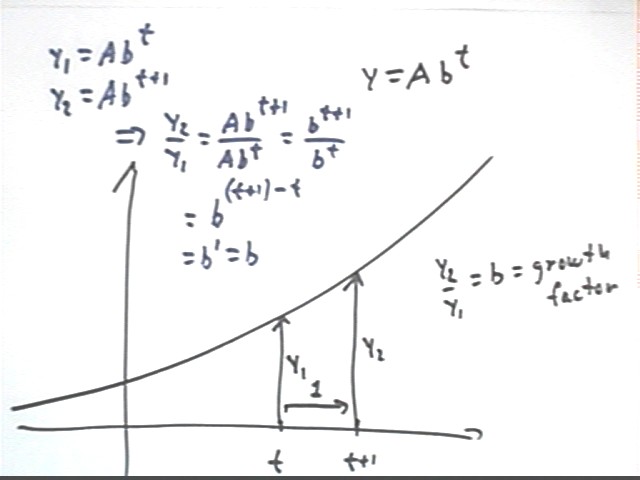
We algebraically prove that for the function y = A b^t, the amount 1 year later is always b times the current amount.
Let t be any time whatsoever.
Then 1 year later the time will be 1 + t.
If we let y1 and y2 be the amounts at times t and 1 + t, we find that
y1 = A b^t and
y2 = A b^(t+1).
Thus the ratio of the two values will be y2 / y1 = A b^(t+1) / A b^t. This expression simplifies, as shown below, to just b. This proves the result.
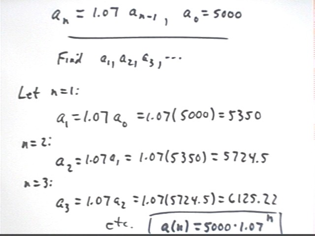
Given the difference equation a(n) = 1.07 a(n-1) with a(0) = 5000, find a(1), a(2), a(3), ... .
First note that in the figure below n and n-1 are indicated as subscripts, not as arguments of functions. This is a standard notation, which is completely equivalent to the function notation we use when typing these expressions.
If n = 1 the equation becomes a(1) = 1.07 a(1-1), or a(1) = 1.07 * a(0). Since a(0) = 5000 we have a(1) = 1.07 * 5000 = 5350.
Similar substitutions allow us to find a(2) from a(1), then a(3) from a(2), etc.
We quickly see that pattern that allows us to conclude that a(n) is obtained by n applications of the factor 1.07, starting with amount 5000, so that a(n) = 5000 * 1.07^n.
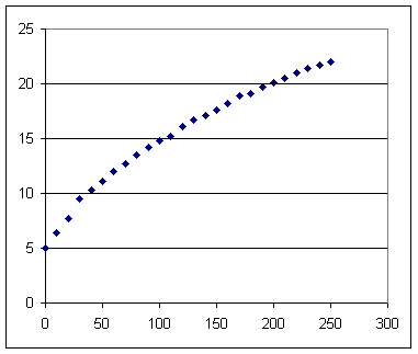
The following observations were made of the temperature reading on a thermometer vs. clock time t. The thermometer was removed from a cold bottle of soft drink, dried and exposed to the air in the room, which was at temperature 25 C.
| Clock Time t (sec) | Temperature T (Celsius) |
| 0 | 5 |
| 10 | 6.4 |
| 20 | 7.7 |
| 30 | 9.5 |
| 40 | 10.3 |
| 50 | 11.1 |
| 60 | 12 |
| 70 | 12.7 |
| 80 | 13.5 |
| 90 | 14.2 |
| 100 | 14.8 |
| 110 | 15.2 |
| 120 | 16.1 |
| 130 | 16.7 |
| 140 | 17.1 |
| 150 | 17.6 |
| 160 | 18.2 |
| 170 | 18.9 |
| 180 | 19.1 |
| 190 | 19.7 |
| 200 | 20.1 |
| 210 | 20.5 |
| 220 | 21 |
| 230 | 21.4 |
| 240 | 21.7 |
| 250 | 22 |
Is the temperature increasing at a constant, an increasing or a decreasing rate.
It's difficult to tell for sure from individual data points, which are a bit uncertain because the instructor who was reading the thermometer really needed to be using reading glasses but wasn't.
However it isn't difficult to see from the temperatures, which were observed at regular intervals, that the tendency is for temperature differences to decrease so that the graph will be increasing at a decreasing rate.
Sketch and describe your graph of temperature vs. clock time, and confirm whether or not the temperature appears to be increasing at a decreasing rate.
A graph of temperature vs. clock time is depicted below. It is clear that the temperatures tend to increase at a decreasing rate, since the tendency of the slope is to decrease as t increases.
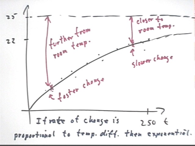
Why do you think that the rate of increase is decreasing?
Most people present said that the closer we get to room temperature the less influence the room temperature has on the temperature of the thermometer. This is an accurate perception.
Physics can refine this perception and make it more precise. It turns out that the influence of room temperature on the temperature of the thermometer is fairly complicated, but to a significant degree of accuracy the rate of temperature change is directly proportional to the difference between the temperature of the thermometer and that of the room.
In the figure below we indicate what this means:
The dotted line at T = 25 indicates the room temperature Troom = 25 C.
The exponential function representing temperature approaches Troom as its asymptote.
When temperature difference is greater the temperature is seen to change at a greater rate.
An exponential function is characterized by the direct proportionality between the excess of the the function value relative to the horizontal asymptote, and the rate of change of that value. Exponential functions arise when this is the case, and every exponential function has this characteristic.
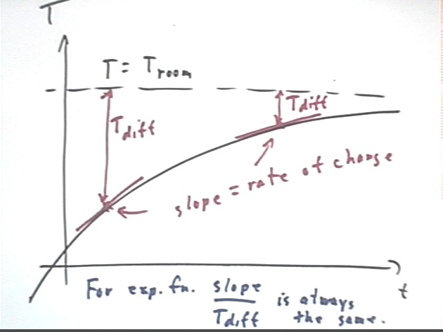
Making the above statements more precise we indicate Tdiff at two points, and the line segments indicating the slopes at those points.
Where Tdiff is greater we see that the slope is greater.
In fact if Tdiff is 3 times as great at one point as at another, the slope should also be 3 times greater at that point than at the other.
This direct proportionality can be indicated by the fact that slope / Tdiff is the same at all points.
Note that this is a direct proportionality, not a proportionality of the square or cube or anything else (i.e., slope / Tdiff is constant, NOT for example (slope / Tdiff)^2 or (slope / Tdiff)^3) ) . It's a proportionality of the first power.
Excel isn't too smart. DERIVE is smarter than Excel but still not smart enough. The curve-fitting algorithm in Excel can only fit an exponential accurately if the asymptote is the x axis. It just can't handle an asymptote at, say, T = 25.
However if we know the asymptote we can trick Excel into giving us what we need.
We note that as temperature approaches its asymptotic value the temperature difference 25 - T shrinks. The temperature difference therefore approaches zero as an asymptote, and Excel can handle this type of data.
The table below is identical to the table given previously except that we have included a column for Tdiff.
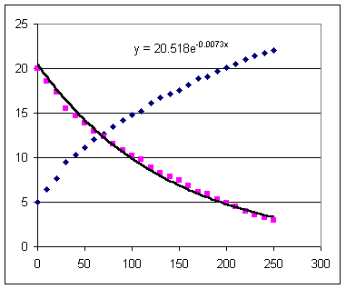
We have included a graph of Tdiff vs. t, indicating the Excel exponential fit
Tdiff = 2-.5 e^-.0073 t.
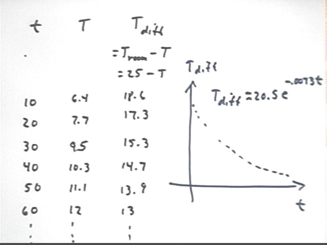
The table below shows all the observed values of Tdiff:
| clock time t (sec) | temperature T (celsius) | Tdiff = 25 - T |
| 0 | 5 | 20 |
| 10 | 6.4 | 18.6 |
| 20 | 7.7 | 17.3 |
| 30 | 9.5 | 15.5 |
| 40 | 10.3 | 14.7 |
| 50 | 11.1 | 13.9 |
| 60 | 12 | 13 |
| 70 | 12.7 | 12.3 |
| 80 | 13.5 | 11.5 |
| 90 | 14.2 | 10.8 |
| 100 | 14.8 | 10.2 |
| 110 | 15.2 | 9.8 |
| 120 | 16.1 | 8.9 |
| 130 | 16.7 | 8.3 |
| 140 | 17.1 | 7.9 |
| 150 | 17.6 | 7.4 |
| 160 | 18.2 | 6.8 |
| 170 | 18.9 | 6.1 |
| 180 | 19.1 | 5.9 |
| 190 | 19.7 | 5.3 |
| 200 | 20.1 | 4.9 |
| 210 | 20.5 | 4.5 |
| 220 | 21 | 4 |
| 230 | 21.4 | 3.6 |
| 240 | 21.7 | 3.3 |
| 250 | 22 | 3 |
The graph below shows T vs. t as before, with T approaching 25, but also shows Tdiff as the decreasing exponential function with asymptote 0.
The graph of the best-fit exponential function is depicted as is the function itself. The function uses y and x to indicate the variables Tdiff and t.
There is another way to 'trick' computer algebra programs such as DERIVE into doing an exponential fit, which is something DERIVE is not designed to do.
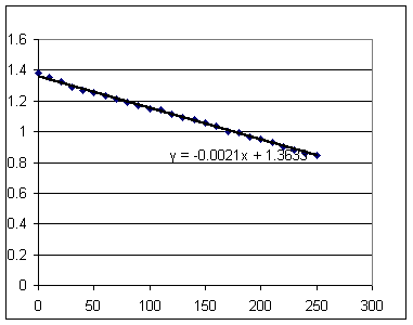
The table below shows log(Tdiff) vs. t. You can verify these values using your calculator and the log key. Calculate the log of the first value Tdiff = 20 and you'll find that you get 1.30 approx., as shown in the table below.
If your data is exponential with asymptote zero then a graph of log(Tdiff) vs. t will result in a nearly straight line.
The table below shows all the Tdiff values for the data we collected.
| t | log(Tdiff) |
| 0 | 1.301029996 |
| 10 | 1.269512944 |
| 20 | 1.238046103 |
| 30 | 1.190331698 |
| 40 | 1.167317335 |
| 50 | 1.1430148 |
| 60 | 1.113943352 |
| 70 | 1.089905111 |
| 80 | 1.06069784 |
| 90 | 1.033423755 |
| 100 | 1.008600172 |
| 110 | 0.991226076 |
| 120 | 0.949390007 |
| 130 | 0.919078092 |
| 140 | 0.897627091 |
| 150 | 0.86923172 |
| 160 | 0.832508913 |
| 170 | 0.785329835 |
| 180 | 0.770852012 |
| 190 | 0.72427587 |
| 200 | 0.69019608 |
| 210 | 0.653212514 |
| 220 | 0.602059991 |
| 230 | 0.556302501 |
| 240 | 0.51851394 |
| 250 | 0.477121255 |
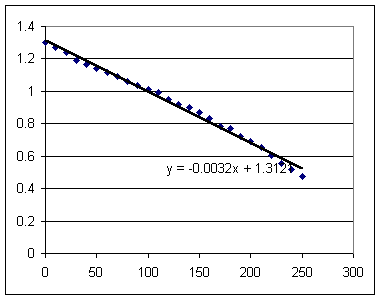
The graph below shows log(Tdiff) vs. t, along with the best-fit straight-line approximation to this data.
log(Tdiff) = -.0032 t + 1.312.
This equation can be solved for Tdiff in terms of t. However the equation involves logarithms, and to solve it will require that we first understand the properties of logarithms.
The solution of this equation, or any equation of this form with the log of one quantity being linearly dependent on another quantity, is an exponential function.
Observe that the data do not give us a perfectly straight line, with values first dipping below, then above, and finally once more below the straight line.
The graph shown below results if we use T = 26 for the room temperature.
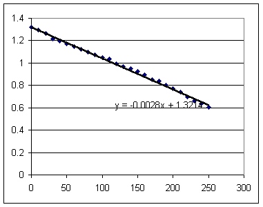
Room temperature T = 27 C gives us an even better fit. However it is unlikely that the temperature was really this high.
Room temperature of T = 28 C and T = 29 C give us the graphs shown below.
Note that while the models appear better these temperatures are definitely higher than those in the room. The 'flattening' of the graph is due to other properties of exponential and linear functions.