Precalculus I Class 03/13
During the preceding class we linearized temperature vs. clock time data by using a log(T) vs. t transformation.
Here we will illustrate the general process we will use in this course to linearize data.
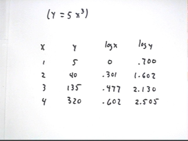
The y vs. x table shown below is built using the y = 5 x^3 function. Usually when we linearize data we don't know what the best function is (as was the case with the temperature data), but for this illustration we'll start with a known function.
Our first step is to create log(x) and log(y) tables, which is easily done using calculator or spreadsheet.
We will then create graphs of log(y) vs. log(x) and log(y) vs. x. A third type of graph we might sometimes use is y vs. log(x), though for this illustration we'll stick to the first two.
A more accurate table is shown here:
| x | y | log x | log y |
| 0 | 0 | ||
| 1 | 5 | 0 | 0.698970004 |
| 2 | 40 | 0.301029996 | 1.602059991 |
| 3 | 135 | 0.477121255 | 2.130333768 |
| 4 | 320 | 0.602059991 | 2.505149978 |
Our graphs will be set up as illustrated below.
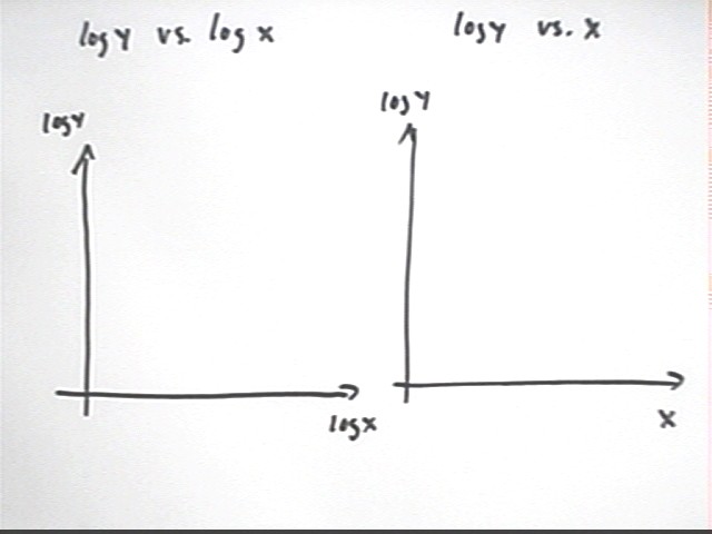
Graph of log(y) vs. x is not very linear, increasing at a decreasing rate:
The graph of log y vs. log x is pretty much linear, increasing at what appears to be a constant rate.
The straight line through these data points has an equation of form log(y) = m * log(x) + b, where m is slope and b is the vertical intercept.
The specific function that fits our graph has slope 3 and vertical intercept .699.
The best-fit function might not be given by your software in appropriate form. Excel, for example, will tell you that the resulting function is y = 3 x + .699. However we know that the graph is not y vs. x but log(y) vs. log(x) so we write this function as log(y) = 3 log(x) + .699.
In the graph below we have changed Excel's y = 3 x + .699 to the more appropriate log y = 3 log x + .699.
Our results correlate with the power function we used to generate the data. We haven't yet developed the tools to see precisely how these relationships exist. However for future reference:
We note that the slope 3 matches the power of the power function y = 5 x^3 we used to generate the data.
Also check out the fact that 10^.699 = 5, which matches the coefficient of our power function.
For reasons that we'll see later, a power function y = A x^p will result in a log y vs. log x graph whose slope is p and whose y-intercept b has the property that 10^b = A.
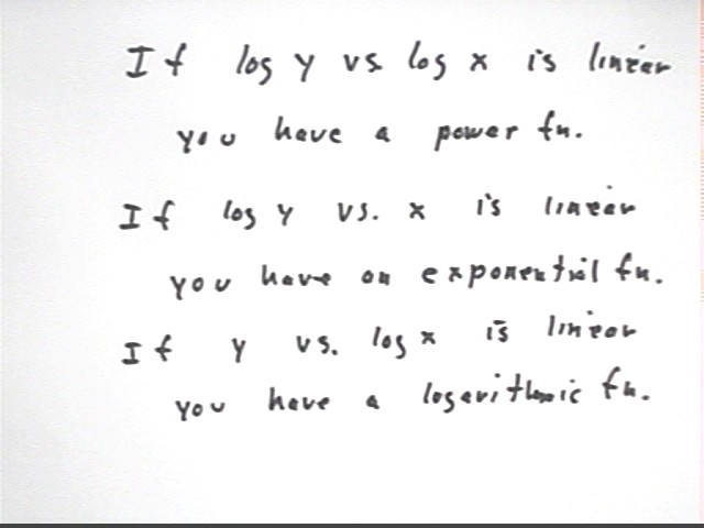
We will see in upcoming classes why the following general rules for linearization hold:
We now investigate the idea of inverse functions.
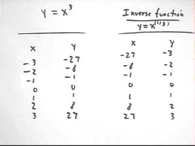
We start with a table for y = x^3.
To get a table for the inverse function we reverse the numbers in the two columns.
Our original function is y = x^3. We obtain the formula for the inverse function as follows:
We first reverse the roles of x and y in the formula y = x^3, obtaining x = y^3.
We then solve the reversed equation for y. We do this as follows:
x = y^3. We take the 1/3 power of both sides, obtaining
x^(1/3) = (y^3)^(1/3). We use laws of exponents to simplify the right-hand side and get
x^(1/3) = y. We switch the two sides to obtain
y = x^(1/3).
We sketch a graph of the function and the inverse function and note its significant characteristics:
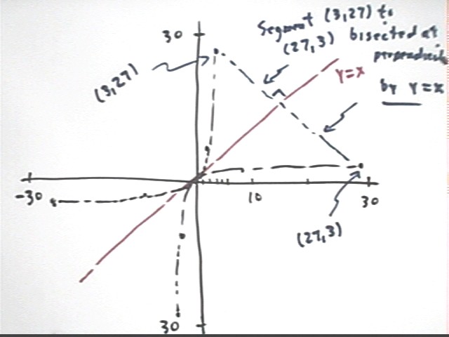
The graph of the inverse function is obtained by reversing the coordinates of the points on the graph of the original function.
The result is that every point on the graph of the original function can be joined to the corresponding point on the graph of the inverse function by a line segment which (provided the graph is drawn with equal scales for the x and y axes) is perpendicular to the line y = x and which is bisected by this line.
For example, (3, 27) on the graph of y = x^3 corresponds to the point (27, 3) on the graph of the inverse function y = x^(1/3). If we join (3, 27) to (27, 3) by a line segment that segment passes through the graph of y = x at a right angle. This segment is bisected (i.e., cut into two equal parts) by the y = x graph.
The main characteristic of a graph of a function and its inverse is that the two functions are symmetric with respect to reflection about the line y = x.
An accurate plot of these functions is shown below:
'Zooming in' on the domain 0 <= x <= 3:
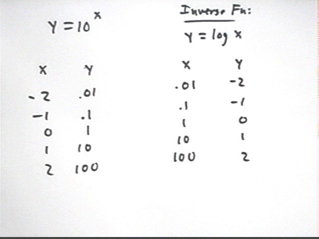
The log function y = log(x) is defined as the inverse of the y = 10^x function.
Note that if we switch coordinates in the expression y = 10^x we get x = 10^y. The equation y = log(x) is therefore equivalent to the equation x = 10^y.
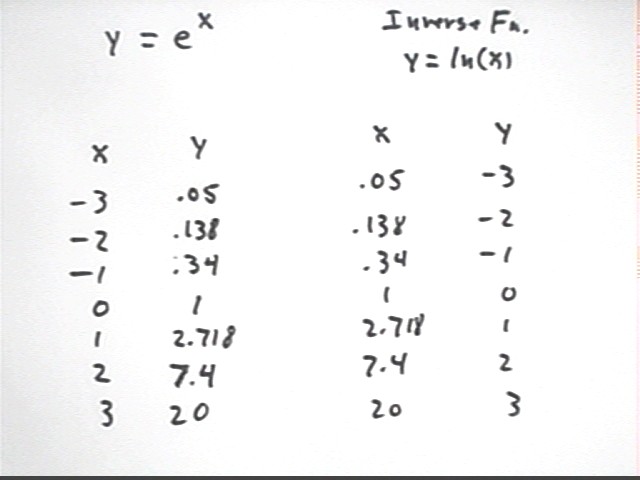
A table of y = 10^x and the 'inverted' table y = log(x) is shown below.
A rough graph of these functions is depicted below. The graph in the lower-left-hand corner is an enlarged graph of these functions near the origin.
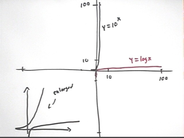
The figure below is a more accurate graph showing y = 10^x, y = log(x) and y = x. Note the symmetry of these graphs with respect to reflection thru the line y = x.
A closeup of the same graphs near the origin shows the following important characteristics:
The graph of y = 10^x passes through (0, 1), is asymptotic to the negative x axis and increases at an increasing rate.
The graph of y = log(x) passes through (1, 0), is asymptotic to the negative y axis and increases at a decreasing rate.
A closeup of the same graphs near the origin shows the following important characteristics:
The graph of y = e^x passes through (0, 1), is asymptotic to the negative x axis and increases at an increasing rate.
The graph of y = ln(x) passes through (1, 0), is asymptotic to the negative y axis and increases at a decreasing rate.
A comparison between the graphs of y = 10^x and y = log(x), and the graphs of y = e^x and y = ln(x), reveals the following:
The x and y intercepts (0, 1) and (1, 0) are the same for the pair y = 10^x and y = log(x), and for the pair y = e^x and y = ln(x).
The graphs of y = e^x and y = ln(x) change more gradually than those of y = 10^x and y = log(x), approaching their asymptotes more slowly and changing curvature more gradually.