Precalculus I Class 03/25
During the preceding class we saw that the power function y = 5 x^3 can be linearized with a log(y) vs. log(x) graph, which has slope 3 and y-intercept .699.
This slope and intercept on the log(y) vs. log(x) graph give us the equation log(y) = 3 log(x) + .699.
We will develop the ideas of logarithms and by the end of class we will see how to solve the equation log(y) = 3 log(x) + .699 for y.
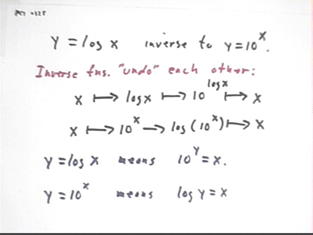
We observe that y = log(x) is the inverse of y = 10^x, as can be verified using a calculator.
If we pick any number for x and use the calculator to find 10^x, if we then take the log of this result we get our original number x back.
If we pick any positive number for x and use the calculator to find log(x), if we then raise 10 to the power of this result we get our original number x back.
You should check these claims out using your calculator.
The figure below shows these relationships schematically. We note the following:
y = log x means the same thing as 10^y = x.
y = 10^x means the same thing as log y = x.
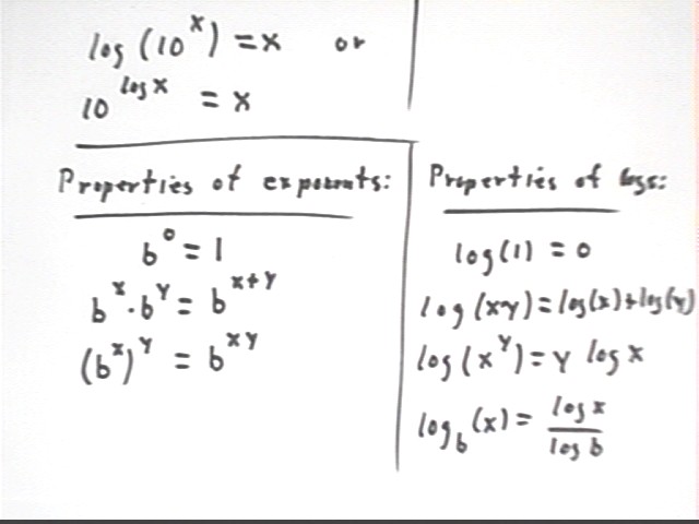
We can also say that 10^(log x) = x, and that log(10^x) = x.
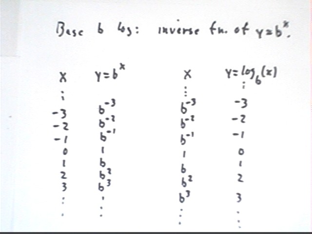
The base b logarithm function is the inverse of the b^x function, as indicated in the table below:
Properties of exponents are related to properties of logarithms, as indicated in the table below.
We can illustrate the law that says that log{base b}(x) = log(x) / log(b) by looking at the relationship between the base-e logarithm ln(x) and the base-10 logarithm log(x):
A table of log(x), ln(x) and log(x) / ln(x) is shown below.
We see that log(x) / ln(x) is always .434, accurate to 3 significant figures.
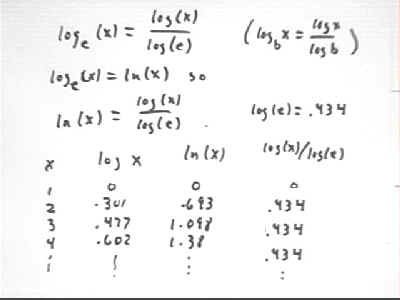
Since ln(x) = log{base e}(x), which by our law is equal to log(x) / log(e), our law tells us that ln(x) should be equal to log(x) / log(e).
You can verify using your calculator that log(e) = log(2.718) is .434 (look again at the table above to see the significance of .434).
Thus log(x) / log(e) = log(x) / .434.
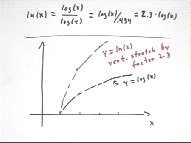
Since 1 / .434 = 2.3, we see that ln(x) = 2.3 * log(x).
This tells us that the function y = ln(x) is a vertical stretch by factor 2.3 of y = log(x).
This relationship is illustrated in the figure below.
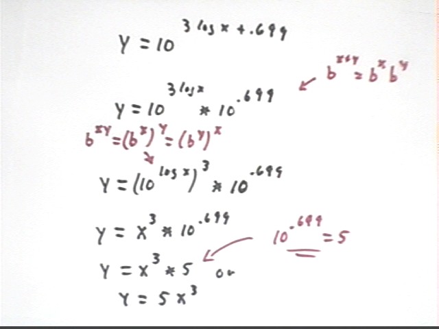
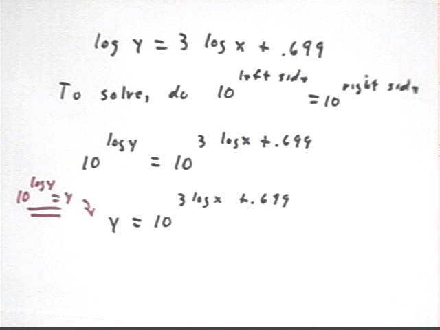
We now use the laws of logarithms to solve the equation log(y) = 3 log(x) + .699.
We begin with the equation log(y) = 3 log(x) + .699, and we raise 10 to a power equal to each side of the equation to obtain the equation
10^(log y) = 10 ^ (3 log x + .699).
Since 10^(log y) = y by the inverse-function relationship we obtain
y = 10 ^ (3 log x + .699).
Starting with y = 10 ^ (3 log x + .699) we complete the solution:
Since b^(x+y) = b^x b^y (where x and y are not related to the x and y in the equation) we have 10 ^ ( 3 log x + .699) = 10^(3 log x) * 10^.699 and the equation becomes
y = 10^(3 log x) * 10^.699.
10^.699 is just a number we can evaluate on our calculator. 10^(3 log x) = (10^(log(x) ) ^3, and 10^log(x) = x so (10^(log(x) ) ^3 = x^3 and we now have
y = x ^ 3 * 10^.699.
Evaluating 10^.699 we obtain 5 so our final equation is
y = 5 x^3.
Note that this is the equation we linearized in the previous class to obtain the equation we just solved. So we've come full circle. The process was:
Linearize the data.
Get the equation of the linearized data.
Solve that equation for y.
In this example we knew the function y = 5 x^3 to start with. Had we not known that the data follows from this equation, we would have found the equation anyway.