Precalculus I Class 04/15
Problem Number 1
Sketch a graph of y = (x - 2.5) ^ 2 (x + 5) (x^2 + 4 x + 3).
There is a second-degree zero at x = 2.5 and a first-degree zero at x = -5.
The quadratic x^2 + 4x + 3 can be factored into (x+3)(x+1), giving us zeros at x = -3 and x = -1. We could also have found these zeros using the quadratic formula, which we should always check if we can't factor the quadratic.
If the polynomial is expanded we get
x^5 + 4·x^4 - 63·x^3/4 - 175·x^2/4 + 275·x/4 + 375/4 =
x^5 + 4·x^4 - 15.75·x^3 - 43.75·x^2 + 68.75·x + 93.75.
The x^5 term takes over for large positive or negative x. For large negative x we see that x^5 is a very large negative number; for large positive x the x^5 terms is a large positive number.
Example of a function that's 'down' at both far left and far right:
If x is a large negative number then x-4 and x-2 are both large negative numbers, but 5 - x is a large positive number so we have three large negative numbers multiplied by a large positive, which gives us a large negative.
If x is a large positive number then x-4 and x-2 are both large positive numbers, but 5 - x is a large negative number so we have three large positive numbers multiplied by a large negative, which gives us a large negative.
Note that the expanded expression is - x^4 + 15·x^3 - 82·x^2 + 192·x - 160. Since the highest-power term -x^4 is the negative of an even power, the result for large positive and negative x will be the negative of a very large positive number, so will be negative.
Important note: - x^4 means - (x^4), since the exponent is applied before the -. If we mean (-x)^4 then we write it with the parentheses.
Problem Number 2
Determine whether the following temperature vs. clock time data are best modeled by an exponential or a y = x^2 power function: Data points are (t, T) = ( 7, 4.65085), ( 7.75, 4.333247), ( 9.75, 3.588362), ( 10.75, 3.26).
Graph
and see which is most nearly linear. Observe the slope m and the vertical intercept b. Write down your equation, which will be
and solve for y. Recall that we usually start by raising 10 to the power of each side, then apply rules of logs to solve.
Problem Number 3
Given the data set ( 4, 5.621661), ( 6, 7.695491), ( 8, 10.53436), ( 10, 14.42048), representing some quantity Q vs. t, find the appropriate transformation or transformations to linearize the corresponding data table. Using either the carefully constructed graph or DERIVE determine the equation of the resulting linear function. Apply the inverse transformation to this function and determine the Q vs. t function which represents the data.
See the answer to problem 2 for an outline of this solution.
The details:
The y vs. x ordered pairs (x,y) are
( 7, 4.65085)
( 7.75, 4.333247)
( 9.75, 3.588362)
( 10.75, 3.26).
In this case log(y) vs. x gives us the most linear of the graphs with points
(7, 0.6675323327)
(7.75, 0.6368134450)
(9.75, 0.5548962489)
(0.75, 0.5132176000).
A straight line fitting the points of this graph will have slope around -.4 and y intercept near 1. You can sketch a graph and see if you can get more accurate results.
With these estimates the graph gives us the function
log(y) = -.04 x + 1.
To solve for y:
10^ log(y) = 10^(-.04 x + 1) so
y = 10^1 * 10^(-.04 x), or
y = 10 * (10^-.04)^x, which we finally put into y = A b^x form as y = 10 * .912^x.
This function gives us y values 5.247638000, 4.897337078, 4.073330730 and 3.714877626. These values are reasonably close to the 4.65, 5.33, 3.59, 3.26 in our data set. However a more accurate estimate of the slope and y intercept of our straight line would give us better results.
Let me know if you have questions, and please remind me in class to mention this solution.
Problem Number 4
For the function y = f(x) = 5 * .8^x, show that the ratio of the average slope to the approximate average value of f(x) is very nearly the same on the interval from x = 3.1 to x = 3.13 as it is on the interval from x = 8.7 to x = 8.73.
We first need to find average slopes and average values on the two intervals.
First evaluate the function at x = 3.1 and 3.13, and at 8.7 and 8.73.
We get respective values 2.503507886, 2.486804608, 0.7175511935, 0.7127637280.
Between x = 3.1 and x = 3.13 the value of x changes by about -.015. The average value is about 2.49. The change in x is 3.13 - 3.1 = .03, so ave rate of change is about -.015 / .03 = -.5.
Between x = 8.7 and x = 8.73 the value of x changes by about -.005. The average value is about .71. Ave rate of change is about -.005 / .03 = -.17.
On the first interval the ratio of the average slope to the approximate average value is about -.5 / 2.49 = -.2, approx.
On the second interval the ratio of the average slope to the approximate average value is about -.17 / .71 = -.23, approx.
The ratios come out pretty close; if you do the calculations with greater precision they come out almost exactly the same.
Problem Number 5
Make a table for y = x^4 for 0 <= x <= 5 and use it to obtain a table for its inverse function. Sketch graphs of both functions and show how the graphs are related. What is the formula for the inverse function? Are there any numbers that the inverse function cannot act on?
| x | y = x^4 | x | y = inv. fn |
| 0 | 0 | 0 | 0 |
| 1 | 1 | 1 | 1 |
| 2 | 16 | 16 | 2 |
| 3 | 81 | 81 | 3 |
| 4 | 256 | 256 | 4 |
| 5 | 625 | 625 | 5 |
Graphs show that inv fn is reflection thru the line y = x of the original function.
The formula for the inverse function is obtained by reversing the roles of y and x in the original formula.
Problem Number 6
What are the basic points of the exponential function y = f(x) = 9 * e^x? Graph the function using these points.
Basic points are the x = 0 and x = 1 points.
f(0) = 9 and f(1) = 9 * e^1 = 9 * e = 24.4.
We plot these two points on our graph and construct an exponential curve asymptotic to the positive or negative x axis, as appropriate.
Problem Number 7
Find Q(1), Q(2), ..., Q(5) for the difference equation Q(n+1) = (1+r) Q(n), with r = -.08008 and Q(0) = 4.
For r = -.08008 we have Q(n+1) = (1 + (-.08008) ) * Q(n-1) = .91992 Q(n-1).
Substituting n = 0 and using our given value of Q(0) we get
Q(1) = .91992 Q(0) = .91992 * 4 = 3.67968.
Substituting n = 1 and using our new value of Q(1) we get
Q(2) = .91992 Q(1) = .91992 * 3.67968 = 3.385011225
Substituting n = 2 and using our new value of Q(2) we get
Q(3) = .91992 Q(2) = .91992 * 3.385011225 = 3.113939526.
A similar calculation gives us Q(4) = 2.864575249, then Q(5) = 2.635180063.
Problem Number 8
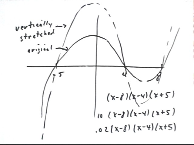
Sketch the graph of a degree 3 polynomial with zeros at x = - 5, 4 and 8, with y taking on increasingly large positive values for large positive values of x.
A degree 3 polynomial has opposite behaviors for large negative and large positive x, so must take increasingly large negative values for large negative x.
A degree 3 polynomial can have only three zeros, and if as in the present case they are all distinct they are all of degree 1, so the graph goes straight thru the x axis at these zeros.
The graph is shown below.
The function could be (x + 5)·(x - 4)·(x - 8) or any positive constant multiple of this expression (e.g., 3 (x + 5)·(x - 4)·(x - 8)). The figure below shows the graph of the 'original' function y = (x-8) ( x-4) ( x+5) along with the graph of this function vertically stretched by a factor of about 2. The stretched graph would be of y = 2 ( x - 8) ( x - 4) ( x + 5). This graph has the same zeros as the original, since moving a point on the x axis twice as far from the x axis just leaves it on the x axis.
Other possible functions, e.g., y = 10 ( x - 8) ( x - 4) ( x + 5) or y = .02 ( x - 8) ( x - 4) ( x + 5), are listed below. They would be obtained from the original by vertical stretches of 10 or .02.
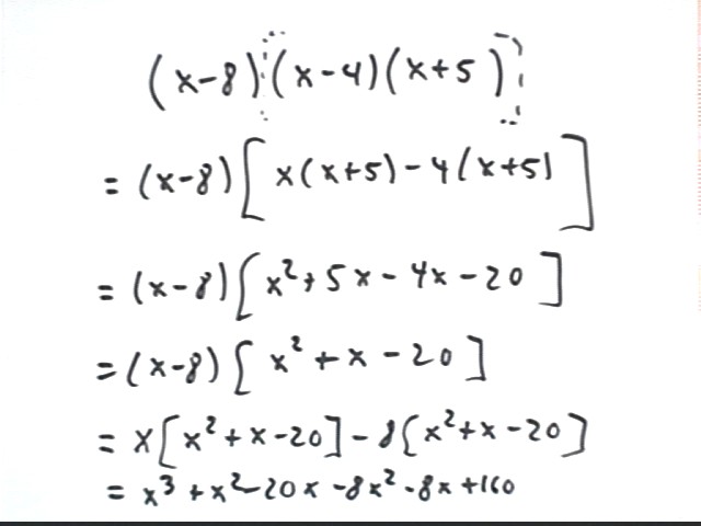
Using (x + 5)·(x - 4)·(x - 8) we multiply out the polynomial:
(x + 5)·(x - 4)·(x - 8) =
(x + 5) [ ·(x - 4)·(x - 8) ] =
(x + 5)· [ x(x-8) - 4(x-8) ] =
(x+5) [ x^2 - 8x - 4x + 32 ] =
(x+5) [ x^2 - 12 x + 32 ] =
x [ x^2 - 12 x + 32 ] + 5 [ x^2 - 12 x + 32 ] =
x^3 - 12 x^2 + 32 x + 5 x^2 - 60 x + 160 =
x^3 - 7 x^2 - 29 x + 160.
The highest-power term is x^3, which dominates the behavior of the polynomial for large positive and negative x. As we have seen, the polynomial is positive for large positive x and negative for large negative x.
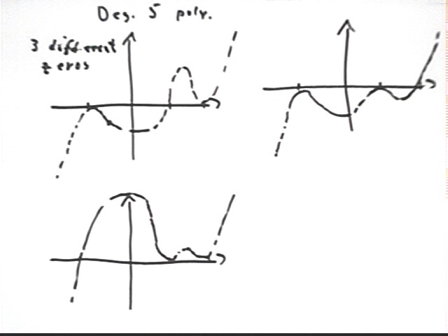
Note: A degree 5 polynomial with exactly three points on the x axis could look a lot like the function give above if it has an irreducible quadratic factor. If a degree 5 polynomial has 5 linear factors and only three different zeros then it might have two degree-2 linear factors to go with a single degree-1 linear factor; or it might have a degree-3 linear factor with two degree-1 linear factors. The figure below shows possibilities a degree 5 polynomial with two degree-2 linear factors. Notes from previous classes show additional possibilities for degree-5 graphs.
Problem Number 11
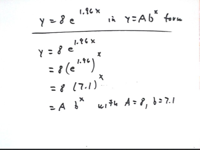
Express the function y = f(x) = 8 * e^( 1.96 x) in the form y = A b^x.
8 e^(1.96 x) = 8 (e^1.96)^x.
Since e^1.96 = 7.1, approx., our function is
8 * 7.1^x.
This is of the form A b^x with A = 8 and b = 7.1.
Problem Number 2a
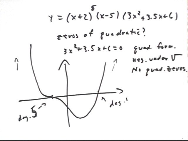
Sketch a graph of y = (x + 2) ^ 2 (x – 5) ( 3 x^2 + 3.5 x + 6).
This graph will have zeros at x = -2 and x = 5, with the first being of degree 2 and the second of degree 1.
We have to check to see whether the quadratic has zeros. Factoring looks hopeless so we use the quadratic formula. We find that the zeros occur at
x = [-3.5 +- sqrt( 3.5^2 - 4 * 3 * 6) ] / (2 * 3).
The discriminant 3.5^2 - 4 * 3 * 6 gives us 12.25 - 48 = -35.75, which is negative. So the quadratic has no zeros.
The quadratic is never 0 so it therefore never changes sign. Since the quadratic is positive for one x value, for example for x = 0, it is positive for all x values.
For large positive x both x + 2 and x + 5 are positive, as is the quadratic, so y will be a very large positive number.
For large negative x both x + 2 and x + 5 are negative, while the quadratic is positive; as the product of a positive and three large negatives y will be a very large negative number.
The resulting graph is shown below on one scale that allows us to see the near-parabolic behavior near x = -2. The lopsidedness of the near-parabola as we move away from x = -2 results from the behavior of the irreducible quadratic, which while never reaching zero has its minimum near x = -.6 and keeps the graph of our function relatively close to the x axis near this minimum.
The graph below uses an expanded y scale, showing us the overall behavior of the function but not really showing the near-parabolic behavior near x = -2.
The exponent of the (x+2) term on the handout given to the class was 5. The graph of the resulting function is constructed in the figure below.
Problem Number 3a
Make tables and sketch graphs of the power functions y = x 2 , y = x 3 , y = x -2 and y = x -3 , for x = -3 to 3.
For y = x^2 and x = x^3 we use the basic points where x = 0 and the points 1 unit right and left of the x = 0 point. For y = x^2 these points are (0,0), (-1,1) and (1,1); for y = x^3 we have basic points (0,0), (-1, -1) and (1, 1).
We also use the auxiliary points where x = 1/2 and x = 2 to help gauge the flatness of the graph near x = 0 and the rate at which steepness increases beyond x = 1.
For y = x^-2 and y = x^-3 we can't use x = 0, since division by 0 is undefined. So we use x = 1 and x = -1, with the auxiliary points where x = 1/2 and x = 2.
You should graph the functions using these points, symmetry properties, and your knowledge of the basic shapes of the graphs.
Then you should construct the vertically stretched graphs by moving each point of the original twice as far from the origin.
The graphs of y = x^2 and y = x^-2 are depicted in two separate graphs below. Each graph is accompanied by the vertically stretched graph. You should verify that each point of the stretched graph lies twice as far from the x axis as the corresponding point of the unstretched graph.
Note that these functions are symmetric with respect to the y axis.
The graphs of y = x^3 and y = x^-3 are depicted in two separate graphs below. Each graph is accompanied by the vertically stretched graph. You should again verify that each point of the stretched graph lies twice as far from the x axis as the corresponding point of the unstretched graph.
Note that these functions have 'reverse symmetry' with respect to the y axis, since an odd power of a negative number is negative. Another way of describing this symmetry is that the graphs are symmetric with respect to the origin.
Problem Number 4a
A population starts at 9000 and grows at the rate of 4.1 percent per year.
The growth rate is 4.1 percent, or .041, when time is measured in years.
The growth factor for this population is 1 + growth rate = 1 + .041 = 1.041.
The function will be
Evaluating this function at t = 1, 2, 3 and 10 we get
Problem Number 5a
Which of the following sequences s1 or s2 is exponential in nature?
An exponential sequence has the properties that its ratios, or the ratios of its first differences, remain constant.
The ratios for the first sequence are
This does not support the hypothesis that this sequence is exponential, since ratios are not constant. We'll go ahead and check the 2d sequence; if those ratios aren't constant then we'll look at ratios of differences.
The ratios for the second sequence are
To a great deal of precision the ratios of the second sequence are constant so we conclude that the second sequence is exponential.
The common ratio 2.2815 is our growth factor.
The process of calculating the ratios of the differences is demonstrated below. We first find the differences between members of the sequence then we calculate the ratios of the differences. If those ratios are the same then the sequence is exponential, corresponding to a basic exponential function y = A b^x vertically shifted by some amount c. Note that if the sequence is in fact exponential the first step, in which we calculate the differences of our sequence, has the effect of canceling out that vertical shift.
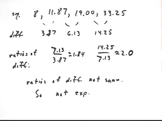
Problem Number 6a
Find the Q(t) vs. t function which best represents the data set ( 7, 441), ( 7.5, 506.25), ( 8, 576), ( 8.5, 650.25). Do this by first finding the appropriate transformation or transformations to linearize the data, then determining the linear function that best fits the transformed data (you may use any means to find this function), and finally using the inverse transformation or transformations to obtain the desired function.
See the nearly identical problem above (#3, and to an extent #2).
Determine which of the three basic transformations best linearizes the data set and proceed as indicated on that problem. The function you end up with here will of course not necessarily be the same function you ended up with previously.
Problem Number 7a
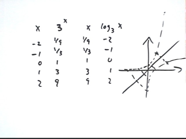
Sketch a graph of log [base 3] (x) vs. x. Show how you obtained this graph without any help from a calculator.
See previous notes on constructing a graph of this type. The procedure is sketched briefly below.
The function log[base 3](x) is the inverse of the exponential function y = 3^x. We construct the graph by first making a table of y = 3^x then inverting the columns to obtain a table for y = log[base 3](x).
We can graph both the exponential and the logarithmic function on the same graph, as indicated in the figure below. These graphs are symmetric with the line y = x.
Problem Number 8a
Determine whether the following temperature vs. clock time data are best modeled by an exponential or a y = x^2 power function: Data points are (t, T) = ( 4, 1.498961), ( 4.75, 1.375422), ( 6.75, 1.153599), ( 7.75, 1.076529).
See the nearly identical problem above (#2).
If your best-fit linear function is log(y) = 2 log(x) + b your function will be a p=2 power function. Your slope might not be exactly 2, but if it's close to 2 then the y = x^2 function is appropriate.
If your best-fit linear function is log(y) = m x + b this indicates an exponential function.
Problem Number 9a
Sketch the graph of a degree 3 polynomial with zeros at x = - 5, 3 and 7, with y taking on increasingly large positive values for large positive values of x.
This problem is nearly identical to a previous problem; only the locations of the zeros and the coefficients of the expanded function differ.
Problem Number 10a
What are the zeros of the linear polynomials f(x) = 4 x - 6 and g(x) = x + 4?
The zeros of the given functions are found by solving the equations
obtaining respective results
The quadratic polynomial is
The quadratic formula tells us that the zeros of this function are
The solutions are identical to the zeros we found from the two linear functions.