class 050831
(refer to matching basic graphs, from 0829)
How do we recognize the three basic points of a linear function based on y = x?
How do we recognize the three basic points of a quadratic function based on y = x^2?
How do we recognize the three basic points of an exponential function based on y = 2^x?
How do we recognize the three basic points of a square root function based on y = sqrt(x)?
According to the depth vs. clock time model:
Is the depth vs. clock time function most clearly related to the linear function y = x, the quadratic function y = x^2, the exponential function y = 2^x or the square root function y = sqrt(x)?
What is the depth at clock time t = 25 seconds?
What is the depth at clock time t = 200 seconds, and what is wrong with this answer?
At what clock time is the depth equal to 25 cm?
What is the minimum depth and when does this occur?
In class we obtained the following information for the depth vs. clock time experiment conducted Monday. The results were averaged over the results obtained by students and represent an approximate weighted mean for each depth:
| clock time (sec) | depth (cm) | depth according to 3-point model | |
| 0 | 90 | 94 | |
| 3.8 | 80 | 80.4 | |
| 7.2 | 70 | 69.2 | |
| 10.4 | 60 | 59.5 | |
| 14 | 50 | 49.7 | |
| 19 | 40 | 37.7 | |
| 24.5 | 30 | 27 | |
| 30.5 | 20 | 18.1 | |
| 41 | 10 | 9.58 |
Using the points (4, 80), (14, 50) and (41, 10) and the form y = a t^2 + b t + c we obtained a system of 3 equations in the unknowns a, b, c and solved the equations, ending up with a = .041, b = -3.74 and c = 94.6. This gives us the model
According to this model the depths at the clock times given in the above table are as given in the fourth column of the table. Each depth was obtained by substituting the corresponding t valud into the 3-point model y = .041 t^2 - 3.74 t + 94.6. We note that the predictions of the model in the fourth column are very close to the observed values.
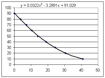
Excel gives us the graph below. The function
was obtained by Excel as the best degree-2 polynomial fit to all the points.
This model takes into account all the points, not just 3 selected points, and fits the data even better than our 3-point model did.

q_a_ Assignment 2.
Overview and Introduction: The Modeling Process applied to Flow From a Cylinder (see also Class Notes #01). Read note below first.
** Note: If so instructed, and only if so instructed, instead of the problems stated in the documents, go to Randomized Problems, Introductory Flow Model (Model 1), and randomly choose one of the nine problem versions. These problems are similar but not identical to those in your documents. **
Completion of the Introductory Flow Model (Class Notes #02) Distance students: submit your solutions to the exercises.
** Continue to use the Randomized Problems from the preceding document. **
Distance Students: View Introduction on CD #2.
When you have completed the entire assignment run the Query program.