synopsis of first week

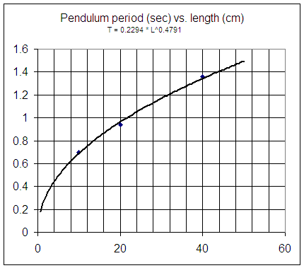
From 15-second counts of pendulums of different lengths obtained in class, we obtain (through a process which is simple enough but which has not yet explained) the following graph, characterized by the function T = .23 L^.48.

We can use the graph to estimate the period of a pendulum of a given length:

• To find the period of a pendulum given its length using the graph we locate the length on the horizontal axis and sketch a vertical line to the curve, then project this straight across to the vertical axis.
• To find the length of a pendulum given its period using the graph we locate the period on the vertical axis and sketch a horizontal line to the curve, then project this straight down to the horizontal axis.

We can obtain period from length, or length from period, using the equation T = .23 L^.48:

• To find the period of a pendulum given its length we substitute the length for L and evaluate the resulting expression for T.  For example if the length is 16 cm we use L = 16 to obtain

T = .23 * 16^.48 = .87.

• If we wish to find the length for a given period we solve T = .23 L^.48 for L by the following steps:

T = .23 L^.48.  Divide both sides by .23 to get

T / .23 = L^.48.  Raise both sides to the power 1 / .48 to get

(T / .23)^(1/.48) = (L^.48) ^ (1/.48).  Since (a^b)^c = a^(bc), (L^.48)^(1/.48) = L^(.48 * 1/.48) = L^1 so we have

L = (T/.23)^(1/.48).  Given a value of T it is possible to enter this expression into a calculator and evaluate it as it is shown here.  However since 1/.48 = 1 / (48/100) = 100/48= 25/12, and since (1/.23)^25/12 = 4.3 ^ 25/12 = 21.4 approx., the form

L = 21.4 T^(25/12), or since 25/12 = 2.08 approx. and since 21.4 is also an approximation,

L = 21.4 T^2.08 are both acceptable simplified forms.

The function T = .23 L^.48 was found using a power-function trendline in Excel.  The algorithm used by Excel to produce this equation is beyond the scope of this course (to understand the algorithm would require a good course in calculus and another in linear algebra).  But we can get a pretty good approximation of the function by solving a set of simultaneous equations, as follows:

• Assume that the function has the form T = A * L^p.

Substitute the coordinates of the data points (.7,10) and (1.35, 40), in turn, into the equation to get

• .7 = A * 10^p and
• 1.35 = A * 40^p.

Divide the second equation by the first to get

• 1.35 / .7 = (A *40^p) / (A * 10^p), which simplifies to give us
• 1.93 = 4^p. 

Use trial and error to estimate p.  (Note that later we will be able to use logarithms to solve for p, but we don't assume at this point that everyone knows how to use logarithms).

We end up with an estimate of p = .47.

Now we plug this valud of p back into the first equation .7 = A * 10^p to get

• .7 = A * 10^.47. 

We easily solve this for A to get

• A = .7 / 10^.47 = .24.

Our model is T = A L^p, or using the values we have obtained for L and p, T = .24 L^.47.