060901
Dave Smith
http://vhmthphy.vhcc.edu/ > physics I > assts (this contains links to worksheets)
Go all the way to the bottom of the assignments page and there's a link entitled Fall 06
http://vhmthphy.vhcc.edu/ > physics I < info takes you to the course of study
Grading Policy (from course of study):
Approximately three tests and a cumulative final examination will be given. The final exam will be weighted as two tests (see weighting below).
A grade will be given on assigned work, based on the student's final mastery of the assignment as evidenced by the initial attempt and followup work based on the critiques received by the student. The average of grades assigned on this work will count as half of a test grade, or approximately 10% of the grade in the course.
Labs must be completed as assigned. The lab average will constitute 25% of the grade for the course.
Both the lab average and the weighted average on tests and exams must be passing in order for a student to receive a grade of C or better.
Raw test and exam scores will be normalized to the following scale, according to the difficulty of the test, as specified in advance of each test by the instructor:
A: 90 - 100
B: 80 - 90
C: 70 - 80
D: 60 - 70
F: Less than 60.
The final grade will be a weighted average of test and exam grades, grades on homework and the lab grade. A summary of the weighting is as follows:
Major Quiz (Physics I only): Weight 0.5 or 1.0, whichever is to the advantage of the student.
Test #1: Weight 1.0
Test #2: Weight 1.0
Test #3 (Physics II only): Weight 1.0
Test #4 (Physics II only): Weight 1.0
Final Exam (Physics I only): Weight 1.0 or 2.0, whichever is to the advantage of the student.
Score on Problems and Questions: Weight 0.5.
Lab Grade: Lab grade is 25% of course grade. Both lab average and the average of all other contributions must both be passing in order to receive a grade of at least C.
Definition of average value on a straight-line graph: On a straight-line graph of A vs. B, the average value of A between two graph points occurs at the midpoint of the corresponding segment of the graph.
On a straight-line v vs. t graph, it follows from this definition that vAve on an interval occurs at the midpoint of the interval.
From this and from the geometry of right triangles, we determine that for a ball rolling from rest, assuming a straight-line v vs. t graph, the average velocity occurs at the midpoint of the time interval which corresponds to motion from one end of the ramp to the other.
This allows us to accurately label the v and t axes of our graph.
Then using any interval we wish, most likely the interval from start to finish, we can determine the acceleration (ave accel is ave rate of change of v with respect to t, which is change in v / change in t:
aAve = `dv / `dt).
Using 2-foot ramps with 1 domino, 2 dominoes and 3 dominoes, and using a pendulum as timer, take the data you need to conduct the above analysis on each ramp.
Write up a summary of how the experiment was conducted, give your data in a table, show the details of your analysis, and list your acceleration vs. number of dominoes at the end.
Determine how far the marble travels on a 2-domino ramp, starting from rest, in 1/2 cycle, 1 cycles, 1.5 cycles, 2 cycles, ... (until you run outta ramp).
Use your data to find average velocity vs. midpoint clock time and construct the corresponding graph of velocity vs. clock time.
Mth 163
Precalculus I
You must have completed Algebra I, Algebra II and Geometry and have a sufficient placement score on the Compass test.
This is a challenging course. Attend every class and figure to start on 5 hours of homework a week. You don't learn mathematics by watching someone do it. You learn by doing it yourself.
The Submit Work form is at http://www.vhcc.edu/dsmith/class_work_form.htm
The homepage for this course is at http://www.vhcc.edu/pc1fall9/ .
Course of Study is under Info at this page. You should read it.
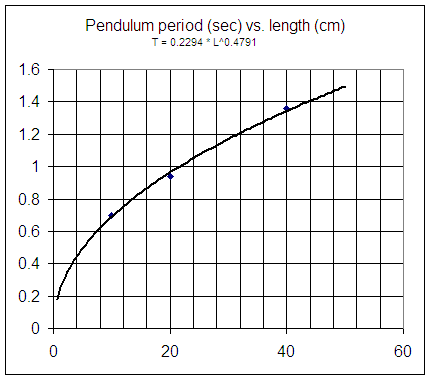
Based on the observations made in one class, here is a graph of pendulum period vs. length. The function that according to this graph relates period and length is
T = .23 L^.48,
approximately, where T is period in seconds and L is length in cm.

According to this graph:
According to the function T = .23 L^.48:
The observed periods for lengths of 15 cm and 40 cm are approximately .7 seconds and 1.35 seconds. If it is known that the period is related to the length by a function of the form T = A * L^p, then
1. Based on this graph estimate the period of a pendulum of length 50 cm and the length of a pendulum with a period of 1.2 seconds.
2. According to the function T = .23 L^.48 find the period of a pendulum of length 55 cm and the length of a pendulum with a period of .8 seconds.
3. According to your best estimates from the graph, is there more change in period between lengths of 15 cm and 25 cm or between 25 cm and 55 cm?
4. According to your best estimates from the graph, does the period of the pendulum change more per additional cm of length between the 10 cm and 25 cm lengths, or between the 25 cm and 55 cm lengths?
5. The observed periods for lengths of 15 cm and 40 cm are approximately .7 seconds and 1.35 seconds. If it is known that the period is related to the length by a function of the form T = A * L^p, then
****
From 15-second counts of pendulums of different lengths obtained in class, we obtain (through a process which is simple enough but which has not yet explained) the following graph, characterized by the function T = .23 L^.48.

We can use the graph to estimate the period of a pendulum of a given length:
We can obtain period from length, or length from period, using the equation T = .23 L^.48:
T = .23 * 16^.48 = .87.
T = .23 L^.48. Divide both sides by .23 to get
T / .23 = L^.48. Raise both sides to the power 1 / .48 to get
(T / .23)^(1/.48) = (L^.48) ^ (1/.48). Since (a^b)^c = a^(bc), (L^.48)^(1/.48) = L^(.48 * 1/.48) = L^1 so we have
L = (T/.23)^(1/.48). Given a value of T it is possible to enter this expression into a calculator and evaluate it as it is shown here. However since 1/.48 = 1 / (48/100) = 100/48= 25/12, and since (1/.23)^25/12 = 4.3 ^ 25/12 = 21.4 approx., the form
L = 21.4 T^(25/12), or since 25/12 = 2.08 approx. and since 21.4 is also an approximation,
L = 21.4 T^2.08 are both acceptable simplified forms.
The function T = .23 L^.48 was found using a power-function trendline in Excel. The algorithm used by Excel to produce this equation is beyond the scope of this course (to understand the algorithm would require a good course in calculus and another in linear algebra). But we can get a pretty good approximation of the function by solving a set of simultaneous equations, as follows:
Substitute the coordinates of the data points (.7,10) and (1.35, 40), in turn, into the equation to get
- .7 = A * 10^p and
- 1.35 = A * 40^p.
Divide the second equation by the first to get
- 1.35 / .7 = (A *40^p) / (A * 10^p), which simplifies to give us
- 1.93 = 4^p.
Use trial and error to estimate p. (Note that later we will be able to use logarithms to solve for p, but we don't assume at this point that everyone knows how to use logarithms).
We end up with an estimate of p = .47.
Now we plug this valud of p back into the first equation .7 = A * 10^p to get
- .7 = A * 10^.47.
We easily solve this for A to get
- A = .7 / 10^.47 = .24.
Our model is T = A L^p, or using the values we have obtained for L and p, T = .24 L^.47.
Quadratic Model
Using the points (4, 80), (14, 50) and (41, 10) and the form y = a t^2 + b t + c we obtained a system of 3 equations in the unknowns a, b, c and solved the equations, ending up with a = .041, b = -3.74 and c = 94.6. This gives us the model
According to this model the depths at the clock times given in the above table are as given in the fourth column of the table. Each depth was obtained by substituting the corresponding t valud into the 3-point model y = .041 t^2 - 3.74 t + 94.6. We note that the predictions of the model in the fourth column are very close to the observed values.
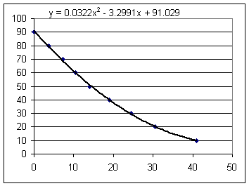
Excel gives us the graph below. The function
was obtained by Excel as the best degree-2 polynomial fit to all the points.
This model takes into account all the points, not just 3 selected points, and fits the data even better than our 3-point model did.
