Precalculus I Class Notes 8/27/98

Quadratic Model of Depth vs. Clock Time (3 points, 3 simultaneous equations)

Here we

• quickly review the properties of a quadratic function,
• go through the details of creating a quadratic model from a set of data and
• compare the model with our data.

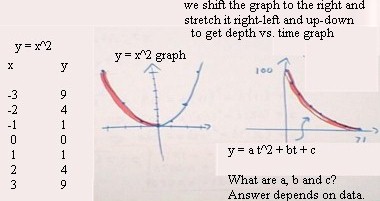
The graph of y = x^2 is a parabola symmetric with respect to the x axis and with its vertex at the origin (0,0). 

We can obtain a graph which very closely models our depth vs. time data (see previous class notes) if we shift this parabola to the right and stretch it in the horizontal (right-left) direction, so it reaches its low point around t = 180 seconds, and in the vertical (up-down) direction so it passes through the y axis around y = 100.

Any parabola can be obtained in this way, and every parabola whose axis of symmetry is vertical will be represented by some quadratic function y = a t^2 + b t + c.   Furthermore every quadratic function will have a parabola as its graph.

To create a quadratic model we can choose three DATA points. 

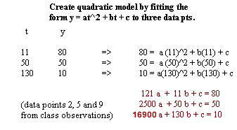
• We have somewhat arbitrarily chosen (11,80), (50,50) and (130,10) from the nine data points obtained previously. 
• We will then substitute these data points into the form y = a t^2 + b t + c of a quadratic function of time.

From the point (11,80), we see that when we substitute 11 for t and 80 for y we obtain the equation 80 = a (11)^2 + b(11) + c. 

• The other points give us, in the same way, the equations we see below. 
• These equations can be simplified into the 'red' set of three simultaneous linear equations (i.e., 121 a + 11 b + c = 80, etc.).

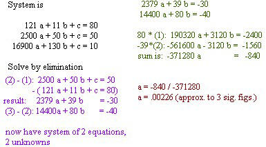
We can solve such a system by any of several methods.  Here we use elimination.

• We see that by subtracting the first equation from the second (the 'purple' set of calculations) we obtain the equation 2379 a + 39 b = -30, and
• by subtracting the second from the third the equation 14400 a + 80 b = -40. 
• We now have a system of two equations in the two unknowns a and b.

This system of two equations is reduced in the 'green' set of calculations. 

• We choose to eliminate b. 
• To do so we multiply the first equation by 80 and the second by -39, so that the coefficients of b are equal and opposite. 
• Then the sum of the two equations give us a single equation, with b eliminated and only a remaining as a parameter. 

We solve the resulting equation for a (the 'red' calculations).

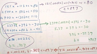
Having obtained a we proceed to obtain the values of b and c by 'back-substitution':

• Substituting a = .00226 into the equation 2379a + 39b = -30 we obtain an equation which we easily solve for b (green arrows and calculations). 
• Then we substitute our values of a and b into the first of the original equations to get c (purple arrow and calculations).

We substitute the values we have obtained for a and b back into the form y = a t^2 + b t + c:

• We end up with the model y = a t^2 + bt + c = .00226 t^2 - .907 t + 89.7.

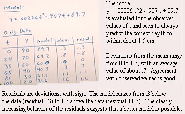
We now evaluate the model to determine how well it fits our original data set:

• We evaluate the model at the observed t values (excepting the ones we chose, which the model will automatically fit perfectly). 
• We obtain excellent, but not perfect, agreement with our data. 
• The steadily increasing pattern to our residuals suggests that by 'tilting' the parabola slightly we could improve the fit.