Precalculus I Class Notes 8/27/98

Quadratic Model of Depth vs. Clock Time (3 points, 3 simultaneous equations)

Here we

• quickly review the properties of a quadratic function,
• go through the details of creating a quadratic model from a set of data and
• compare the model with our data.

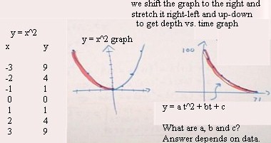
By stretching and shifting the graph of the basic parabola y = t^2, we can obtain the graph of any quadratic function y = a t^2 + b t + c. To fit a quadratic function to our depth vs. clock time data, we choose three points we believe to lie on the graph of depth vs. clock time. We substitute the coordinates of these points into the form y = a t^2 + b t + c to obtain three simultaneous linear equations in the parameters a, b and c. We solve these equations using elimination to obtain a, b and c which we then substituting to the form y = a t^2 + b t + c to obtain our quadratic model. We then evaluate the model by evaluating y each t value from our original data set, and compare these predictions of the model with the actual observe y values. The differences between predicted and observe values are called 'residuals'; we consider our model to be good if residuals are small and if there is no consistent pattern to the residuals.

The graph of y = x^2 is a parabola symmetric with respect to the x axis and with its vertex at the origin (0,0). 

We can obtain a graph which very closely models our depth vs. time data (see previous class notes) if we shift this parabola to the right and stretch it in the horizontal (right-left) direction, so it reaches its low point around t = 180 seconds, and in the vertical (up-down) direction so it passes through the y axis around y = 100.

Any parabola can be obtained in this way, and every parabola whose axis of symmetry is vertical will be represented by some quadratic function y = a t^2 + b t + c.   Furthermore every quadratic function will have a parabola as its graph.

To create a quadratic model we can choose three data points. 

• We have somewhat arbitrarily chosen (11,80), (50,50) and (130,10) from the nine data points obtained previously. 
• We will then substitute these data points into the form y = a t^2 + b t + c of a quadratic function of time.

From the point (11,80), we see that when we substitute 11 for t and 80 for y we obtain the equation 80 = a (11)^2 + b(11) + c. 

• The other points give us, in the same way, the equations we see below. 
• These equations can be simplified into the 'red' set of three simultaneous linear equations (i.e., 121 a + 11 b + c = 80, etc.).

We can solve such a system by any of several methods.  Here we use elimination.

• We see that by subtracting the first equation from the second (the 'purple' set of calculations) we obtain the equation 2379 a + 39 b = -30, and
• by subtracting the second from the third the equation 14400 a + 80 b = -40. 
• We now have a system of two equations in the two unknowns a and b.

This system of two equations is reduced in the 'green' set of calculations. 

• We choose to eliminate b. 
• To do so we multiply the first equation by 80 and the second by -39, so that the coefficients of b are equal and opposite. 
• Then the sum of the two equations give us a single equation, with b eliminated and only a remaining as a parameter. 

We solve the resulting equation for a (the 'red' calculations).

Having obtained a we proceed to obtain the values of b and c by 'back-substitution':

• Substituting a = .00226 into the equation 2379a + 39b = -30 we obtain an equation which we easily solve for b (green arrows and calculations). 
• Then we substitute our values of a and b into the first of the original equations to get c (purple arrow and calculations).

We substitute the values we have obtained for a and b back into the form y = a t^2 + b t + c:

• We end up with the model y = a t^2 + bt + c = .00226 t^2 - .907 t + 89.7.

We now evaluate the model to determine how well it fits our original data set:

• We evaluate the model at the observed t values (excepting the ones we chose, which the model will automatically fit perfectly). 
• We obtain excellent, but not perfect, agreement with our data. 
• The steadily increasing pattern to our residuals suggests that by 'tilting' the parabola slightly we could improve the fit.