"
Class Notes Precalculus I, 9/15/98
Rates; Modeling by a Linear Function
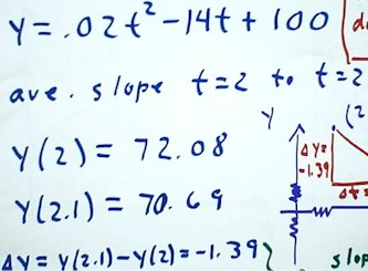
The quiz problem for today was to determine the average slope of the graph
of the depth vs. time function y(t) = .02 t^2 - 14 t +
100, between clock times t = 2 and t = 2.1.
- We assume that depth is in cm and time
in seconds.
- We begin by determining the depths at the two clock times,
by substituting t = 2 and t = 2.1 into the definition
of y(t).
- We obtain y(2) = 72.08 and y(2.1) = 70.69.

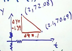
Since we are determining the slope, we sketch a graph of y vs.
t.
- The two graph points are
depicted in the figure below.
- The rise from the
first point to the second is easily found to be `dy
= 70.69 - 72.08 = -1.39, representing the 1.39 cm decrease in depth,
and the run is easily found to be `dt = .1, representing
the .1 second time interval between the first point and
the second.
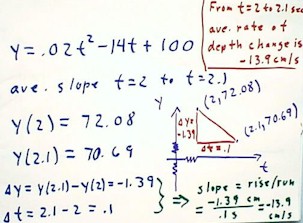
- The slope will be
easily found as rise / run = `dy / `dt.
We easily calculate the slope `dy / `dt = - 13.9 cm / sec, which
represents the average rate at which water depth changes between
clock times t = 2 and t = 2.1 seconds.
- The note at the upper right hand
corner of the figure below indicates this interpretation.
Video Clip #01
http://youtu.be/nuI_Kz5x0hs
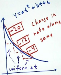
An important property of quadratic functions is that
if we calculate the average rate of change over a series of
connected intervals, using the same `dt for each
interval, the change in rate will always
be the same from one interval to the next.
- The figure below shows rates
which increase by 8 from one interval to
the next.
- The next rate would
be +4, though this value doesn't correspond very well with the picture.
Video Clip #02
http://youtu.be/6onIszfV9gw
When we take the slope between two points of the graph
of y vs. t, we are representing an average
rate of change between the two values of t.
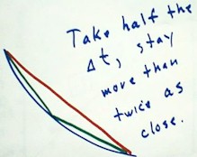
- The red line segment between
two points of the curved blue graph below gives us an average
rate over the extended time interval between the two
points.
- If we cut the time
interval in half, we obtain average rates corresponding
to the the two green segments.
- Note how the green
segments stay much closer to the curve then the
red segment. In fact, though we cut the length of
the t interval in half, the green segments are
more than twice as close to the curve, on the average.
- So for twice the work (calculating
two slopes instead of 1) we obtain more than twice the accuracy.
- This is an important
property of slopes of smooth curves.
- This idea will occur in greater
depth when and if you take a course in calculus.
Video Clip #03
http://youtu.be/xymarqZHAxY
Video Clip #04
http://youtu.be/68vsBaIXvtM
In-class observations of the distance below a lab table (the
'spring reading' on the graph) of a milk jug suspended from a spring,
vs. the number of cups of water added to the milk jug,
gave us the points
(3 cups, 44.7 cm), (6 cups, 47.8 cm), (9 cups, 52.3 cm), (12 cups, 57.2 cm), and (15
cups, 61.7 cm).
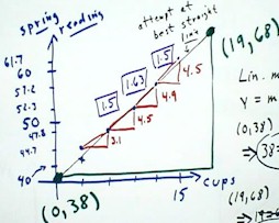
- When these points are plotted on a graph, we see that
the last four points very nearly lie on a straight line,
since the average slopes of the graph in the three intervals defined
by those points are nearly the same.
- We noted that for the first few cups this spring didn't extend
much, so we discount the first point.
- We attempt to fit a straight line to the last four points,
in the sense that we try to find the line which minimizes the
average distance from the four points.
- (Actually what we ultimately try to do is minimize the average of the squared
vertical distances between the points and the line, but the reason for that is a
subject for a statistics class or, at a more advanced level, for a calculus class).
- The figure below shows a halfway reasonable but not very accurate attempt to sketch
such a straight line. We will attempt to find the equation
of this line.
- Having obtained the line we estimate the coordinates of two
points on the line.
- We choose two points as
far apart as practical to minimize the effect of
any unavoidable error we might make in estimating their coordinates.
- In-class estimates for
these points were (0,38) and (19,68).
Video Clip #05
http://youtu.be/FLJf7fMspzY
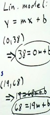
Having found two points to define the line,
we simply plug the coordinates of the points into the form
y = mx + b of the general linear function.
- We obtain two equations, 38 = 0m + b (or just 38 = b) and 68 = 19m + b.
- We can easily solve these two equations as a system
of simultaneous linear equations, obtaining b = 38 and
m = 30/19 (approximately 1.55).
We interpret the resulting function y(x) = 1.55x + 38 by noting that
the slope 1.55 represents the rate 1.55 cm / cup at
which the position of the milk jug changes with respect
to the amount of water added.
- Since y(0) = 38,
we conclude that the position of the milk jug when zero
cups of water have been added (i.e., when the jug was empty) must have been 38
cm.
http://youtu.be/6fvGR2KKvDI
"
