Exponential Functions

Class Notes Precalculus I, 10/20/98

Exponential Functions

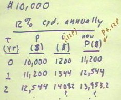
The figure below shows how $10,000 compounded annually will grow.

The columns show the time t in years from the initial investment, the principle P at time t, the interest earned during the year beginning at time t, and the new principle at the beginning of the next year. The calculations are straightforward.
The interest i is just .12 P, and the new principle is just P + .12 P, representing the old principle plus the interest earned.

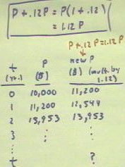
The algebraic expression for the new principle P + .12 P can be simplified by factoring out P to obtain P (1 + .12), then by adding the numbers in parentheses to obtain 1.12.

The final expression for the principle is 1.12 P.

We can thus redo the table, using columns for t, P and the new principle 1.12 P.

We raise the question of what the principle will be after t years.

Note error: for t = 2, P is listed as 13,953; it should be the 12,544 found in the previous line.

Video File #01

http://youtu.be/zlgOCEstbjA

Once again we redo the table.

At the end of the first year our principle will be 1.12 * $10,000
At the end of the second year we will have multiplied the principle by 1.12 again, so that we have 1.12 ^ 2 * $10,000.
Multiplying by 1.12 at the end of the third year we obtain principle 1.12^3 * $ 10,000.

An obvious pattern has been established.

At the end of t years, we will have multiplied $10,000 by 1.12 a total of t times, so we will have principle 1.12^t * $10,000.

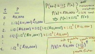
We therefore say we have the principle function P(t) = $10,000 (1.12)^t.

We identify the $10,000 as the initial quantity, the 1.12 as the growth factor (a factor is something we multiply by), and the.12, corresponding to the 12 percent, as the growth rate.
We must be careful not to confuse growth rate with rate of change; a rate of change quantity y with respect to t is the ratio `dy / `dt, representing the change in the quantity y per unit of change of t.
A growth rate is a factor by which we multiply a quantity to get the change in the quantity itself.

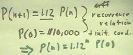
The recurrence relation P(n+1) = 1.12 * P(n) tells us that to get the quantity P at step n+1, we must multiply the quantity at step n by 1.12.

This is in fact what we did with our principle at the end of each year to get the principle at the end of the next year.

In this case each step represents another year.

If we combine this recurrence relation with the initial condition P(0) = $10,000, then

we obtain P(1) = 1.12 * P(0) = 1.12 * $10,000 = $11,200,

then using this result we obtain P(2) = 1.12 * P(1) = 1.12 * $11,200 = $12,544, which we then used to find P(3), etc..

The net result is that to get P(n), we multiply P(0) by 1.12 at total of n times, with the result that P(n) = 1.12 ^ n * P(0).

Video File #02

http://youtu.be/KTmHLICoydQ

In general an exponential function is represented by an initial quantity Q0 and a growth factor b, giving us Q(t) = Q0 * b^t.

In some cases there will also be a constant number c added to this expression. This constant number could, for example, represent $100,000 buried in the back yard, while Q0 b^t represents the value of our investment Q0 which grows according to the growth factor b (e.g., our $10,000 with growth factor 1.12).

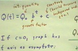
If c = 0, our graph of Q vs. t has the t axis as an asymptote.

A positive growth rate will give us a growth factor b > 1 so that b^t approaches zero as t becomes more and more negative.
A negative growth rate will give us a growth factor b < 1, so that b^t approaches zero as t becomes more and more positive.
In either case the graph approaches the t axis.

For a positive growth rate, depicted by the graph below, the time for the quantity Q to double can be represented by an interval of width tDoub, as shown below.

In this picture Q doubles from Q1 to 2 Q1 (Q1 has erroneously been labeled Q0 in red; Q = Q0 is in fact the Q intercept of the graph), as labeled in red, as the clock time changes from t0 to t0 + tDoub.
That is, starting at clock time t0, a time change of tDoub results in a doubling of Q.

If the quantity at time t is Q(t), the quantity at t0 is just Q (t0), and the quantity after time tDoub has passed is Q(t0 + tDoub).

Since the second quantity represented doubling of the first, we have Q(t0 + tDoub) = 2 Q(t0).

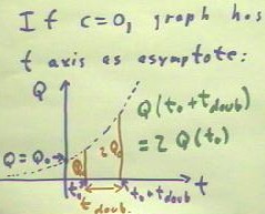
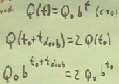
We can represent this situation by writing the equation in terms of the function Q(t) = Q0 b^t.

For this function, Q(t0 + tDoub) = Q0 b^(t0 + tDoub) and Q(t0) = Q0 b^t0, so the equation Q(t0 + tDoub) = 2 Q(t0) becomes Q0 b^(t0 + tDoub) = 2 Q0 b^t0.

Video File #03

http://youtu.be/GebZ_RxC8dM

The picture below represents again the fact that Q(t0 + tDoub) = 2 Q(t0).

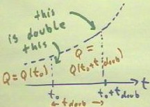
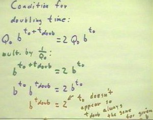
We now solve the equation Q0 b^(t0 + tDoub) = 2 Q0 b^ t0, for t0.

We see that we can eliminate Q0 from the entire equation by multiplying by its reciprocal 1/ Q0, obtaining b^(t0 + tDoub) = 2 b^t0.

We can then apply the laws of exponents to write the left-hand side as b^t0 * b^tDoub.

Finally we multiply both sides by 1 / b^t0 to obtain b^tDoub = 2.

We note that in this expression b^tDoub = 2 for tDoub, the initial time t0 never appears.

Thus the doubling time tDoub must be the same for every starting time.

http://164.106.222.225/pc1spring99/lectures/pc_981013_981029/pc1_1020/class_ notes.htm

To solve the equation b^tDoub = 2 for tDoub, we can use either trial and error, which is the only option open at this time, or we can use logarithms, as we will see next week.

The main point here, however, is that for any growth factor b associated with a positive growth rate r, we will have a well-defined doubling time which applies to any starting point.
Therefore the doubling time doesn't depend on the quantity Q or on the starting time t0.

Video File #04

http://youtu.be/Sw4QwHFC-Hg