Linearizing Data

Class Notes Precalculus I, 11/10/98

Linearizing Data

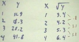
The quiz problem for today was to attempt to linearize the y vs. x data in the figure below, first by using the transformation y -> `sqrt(y) then by using the transformation y => log(y), and to compare the results of the two linearizations.

We first use the `sqrt(y) transformation, taking the square roots of all the y values to get the table at right in the figure below.

A quick check shows that the first difference sequence of the y values is .8, 1.1, 1.1.
If the linearization has succeeded, these differences should then be uniform; this might or might not be the case here.

This sequence appears to have a tendency to increase, but this appearance could be due to random fluctuations in data.

If there were more data points it would be easier to determine whether there is in fact a tendency for the differences to increase, or whether the apparent increase in differences is due to unavoidable random fluctuations.

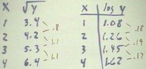
We next attempt to linearize linearize the data using the log function, and obtain the second table below.

The difference sequence is .18, .19, .17, which is much more consistent than before.
These differences seems much more likely than that obtained in the previous attempt to be the result of random fluctuations around a constant value, as opposed to being the result of choosing the wrong model.

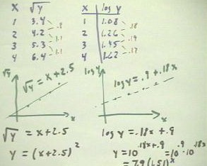
We next sketch graphs of the two attempted linearizations, obtaining graphs something like those shown below (you should make your own graphs to see for yourself how their shapes are related to the tables, and particularly to the differences found on the two tables.

We fit each graph with an approximate best-fit line (DERIVE would give us the best possible linear fit).
The estimates we obtain for these best fits are

`sqrt(y) = x + 2.5 and

log y = .18 x + .9

These estimates can be obtained by estimating slope and y intercept or by determining the coordinates of two points on each best-fit line and using these points to obtain the corresponding linear models. You should make your own estimates.

Having obtained the linear functions corresponding to each graph, we then solve each for y to obtain the y vs. x model.

We easily solve the first equation by squaring both sides.
We obtain y = (x + 2.5)².

We solve the second by using the fact that log y = a means that y = 10^a, thus obtaining from log y = .18 x + .9 the equation

y = 10^{.18 x + .9}.

We simplify this first using the exponential law x^ab = x^a x^b, obtaining 10^.9 * 10^.18x.
10^.9 is about 7.9 and 10^.18x = (10^.18)^{^x} = 1.51^x (approximately).
Our model will therefore be

y = 7.9 (1.51)^x.

Video file #01

http://youtu.be/I-ZpHL-fgMo

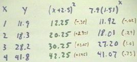
We finally compare our two models with the original data.

The table below depicts the original data and the results of using the y = (x + 2.5)² model (3d column, in green) and the y = 7.9 (1.51)^x model (fourth column, in blue).
Next to each column, in red, are the residuals, the differences between the model and the original data.
We note that, while the first model stays reasonably close to the data, its residuals fluctuate much more than those of the second model, and are considerably greater in magnitude.

We therefore conclude that the second model is more appropriate to the data.

However, these models have been obtained by the instructor's eyeball estimates based on the graphs shown above; you should validate these models by your own eyeball estimates based on your own graphs, and you should also use DERIVE to obtain the actual best-fit straight lines for the transformed data and obtain the corresponding models.

Note error in figure: Note that the last three residuals indicated for the (x + 2.5)² model are labeled as positive. These residuals are negative, since the original y is in each case below that predicted by the model.

Video file #02

http://youtu.be/9ZzN8eNlGCc

Video file #03

http://youtu.be/clYmChnY1FY

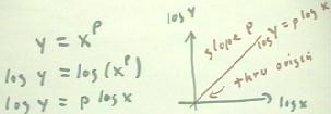
We next observe that if we transform the function y = x^p by taking the log of both sides, we obtain log y = p log x.

If we graph this equation on a set of log y vs. log x coordinate axes, we see that the vertical coordinate is just p times a horizontal coordinate.

The graph is therefore a straight line through the origin of the log y vs. log x axes, with slope p.

Had we applied the same transformation to the more general power function y = A x^p, we would have obtained log(y) = p log(x) + log(A), as you should verify using the laws of logarithms.

Since log(A) is just a constant number, as is the power p, we see that this equation is analogous to that of the general linear function y = mx + b.
Therefore when we graph log (y) = p log (x) + log (A) on a log y vs. log x set of coordinate axes, we will get a straight line with slope p and y intercept A.

Thus by transforming data corresponding to a power function by the transformation x -> log x and y -> log y, we will obtained a graph whose y intercept is log (A) and whose slope is p, for the model y = A x^p.

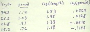
In class we measured the period of a pendulum as a function of its length.

To do so we allowed a pendulum to swing freely back and forth while we counted 10 completes cycles of its motion, and using a computerized timer determined the length of time required for each swing.
This length of time is called the period of the pendulum.

Taking the word of the instructor that physics ensures that this data should very accurately modeled by a power function of the form y = A x^p, we then proceeded to transform both the length and the period data using the transformations length -> log (length) and period -> log (period). We obtained the values in the table below.

Video file #04

http://youtu.be/N2Ac6Os36bk

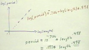
A sketch of the graph of the transformed data is shown below as a graph of log (period) vs. log (length).

We could have estimated the slope in y intercept of this graph, but since this date is expected to be very accurate we used DERIVE to obtain the best-fit line

best-fit line for log(period) vs. log(length): log (period) = -.706 + .498 * log (length).

Solving this equation for period, we obtained

period = 10^{-.706 +.498 * log (length)}.

To obtain this solution we used the laws of logarithms in the usual manner to obtain. = 10^-.706 * 10^{.498 * log (length)} =.197 * (10^{log (length)^.498}) =.197 * length ^.498.

Physics tells us that the period of the pendulum should be (`sqrt(length / 980) * 2 `pi) = `sqrt(length) * 2 `pi / `sqrt(980) = `sqrt(length) * 6.28 / 31.2 = .200 * length^.5.

Comparing period = .200 length^.5 with our model, we see that our value of .197 is close to the theoretical value of .200, and our value of .498 is similarly close to the theoretical value of .500.
Our model deviates from the theoretical model by an amount that is easily explained by the fact that our computer timing program has an inherent inaccuracy of approximately .03 seconds, and that of the computer timing program was triggered by a human observer responding to the command of another human observer, a situation which brings the inherent inaccuracy of the timing process to approximately .1 second.
The .1 second uncertainty of the times in our original table is more than enough to explain the slight discrepancy between our .197 and the 'ideal' value .200, and between our .498 and the 'ideal' value .500.

Video file #05