Quadratic modeling problems in which you are to
select three points from a graph of a smooth curve which approximately models data derive three simultaneous equations for the parameters of the quadratic model
write the specific quadratic function and
use that function to answer various questions about the behavior of the model (e.g., where is the function zero, where is it a maximum or minimum, what is y for a given x, what is x for a given y?).
Problems related to the graph of a quadratic:
finding the zeros and the coordinates of the vertex for a given function
finding the parameters a, b, c of the ax^2 + bx + c model for a given graph
Function notation questions
for given f(x) find f(`expression), where `expression can be any algebraic expression
for the graph of an unspecified function f(x) use the f(x) notation to show how to find f(x) for a given x, or to find the x for which f(x) takes a specified value
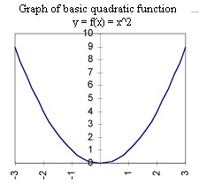
Graphs of the basic functions
be able to quickly construct the graph of the basic form of a linear, quadratic, exponential or pth power function
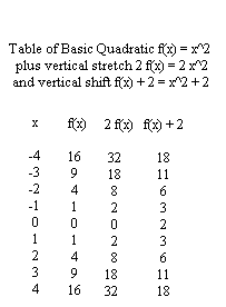
if f(x) stands for the basic linear, quadratic, exponential or pth power function, construct a table and graph for a f(x), f(kx), f(x-h), and/or f(x) + c for specified values of a, k, h and/or c
Rate and slope calculations
for a given set of data calculate the average rate associated with each pair of consecutive points and show how these rates appear on the graph
for a specified function f(t) obtain a table of values to a given set of equally spaced t values, and calculate the associated rates; graph the values on the table and show how the rates appear on the graph
given the graph of a function y = f(x) and the units of y and x, determine the units of the rate and/or the slope (e.g., if y is depth in cm and x is time in sec, slope is the rate in cm/sec at which depth changes)
Summary of Modeling Process, Version 2 You should be thoroughly familiar with this process. Besides having memorized the steps, you should be able to describe how each step was applied to the quadratic model of depth vs. time.
Orient
Predictions, speculations.
Observe
Set up and take data.
Organize Data
| time | depth |
30 |
49 |
60 |
16 |
90 |
1 |
Graph
Postulate
quadratic function depth = a t^2 + bt + c ????
Select Representative Points

Obtain an equation for each selected point
400 a^2 + 20 b + c = 611600a^2 + 60 b+ c = 13
8100a^2 + 90 b+ c = 2
Solve the system of equations
a = .01, b = -2, c = 100Substitute parameters
depth = .01t^2 - 2 t + 100Graph the model

Quantify the comparison
Average of deviations = 2.43Pose and answer questions

Do the science: relate the mathematics to the real world.
Pressure is proportional to depth.
Energy conservation implies that velocity is proportional to square root of pressure.
Thus dy/dt = k `sqrt(y).
Therefore velocity is quadratic in time.

Basic function: y = x^2
Generalized function:
y = f(x) = ax^2 + bx + c (quadratic formula form)
or, alternatively,
y = f(x) = a(x-h)^2 + c (standard form)
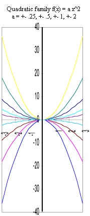
Function family:
Key parameters:
Vertical stretch factor a (both forms)
** Need not know for first test ** Horizontal shift h (standard form f(x) = a(x-h)^2 + c); also x coordinate of vertex
** Need not know for first test ** Vertical shift c (only for standard form f(x) = a(x-h)^2 + c); also y coordinate of vertex for this form only
Key characteristics of graph:
Shape of a vertical parabola
Symmetry with vertical axis through vertex
Slope of graph changes at a constant rate
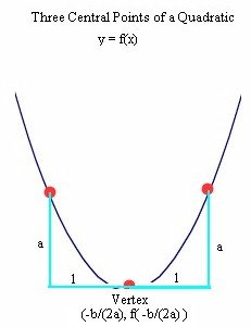
Key points for graphing:
Vertex: xVertex = -b/2a, yVertex = f (xVertex)
Zero(s): x = [ -b +- `sqrt(b^2-4ac))] / (2a), whenever b^2-4ac >= 0
1 unit right and left of vertex: (xVertex+1, yVertex+a) and (xVertex-1,yVertex+a)
Typical situations:
Depth vs. time for flow from a uniform cylinder
** Need not know for first test ** Altitude of a thrown ball vs. time
** Need not know for first test ** Revenues vs. selling price (simplified economic model)
** Need not know for first test ** Curvature-based approximation to any continuously changing quantity over a short time interval
Rate equation:
** Need not know for first test ** d [dy / dt] /dt = constant (rate of change changes at a constant rate)
** Need not know for first test ** dy / dt = k `sqrt(y)
Difference equation:
** Need not know for first test ** a(n+1) = a(n) + c n
Sequence behavior:
** Need not know for first test ** Sequence f(n) has linear first difference, constant second difference
f(x) notation
If f(x) represents a function, f(`expression) represents that function with every x replaced by `expression.
For example if f(x) = 2x^2 - 3, f(4) indicates that x has been replaced by 4, so f(4) = 2(4^2) - 3. f(x+3) indicates that x has been replaced by x+3, so f(x+3) = 2(x+3)^2 - 3. f(x) - 4 indicates that x has been replaced by itself, so we have f(x) - 4 = (2x^2 - 3) - 4.
To find f(x) for a given x, given a graph of f(x), we locate x on the x axis, move vertically up or down to the curve, then horizontally across to the y axis. To find the x for a given value of f(x), locate that value on the y axis, move horizontally across to the curve, then vertically up or down to the x axis.
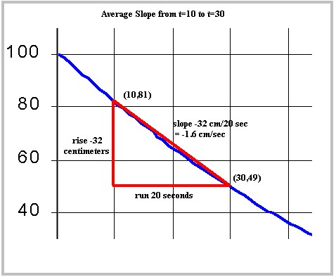
Rate and Slope Calculations If depth changes from 81 cm to 49 cm between clock times 10 sec and 30 sec, then we have a depth change of -32 cm in a time interval of 20 sec. The average rate at which depth changes is therefore -32 cm / 20 sec = -1.6 cm/sec.This situation is depicted graphically by a curve passing through the points (10,81) and (30,49) on a graph of depth in cm vs. time in sec. The depth change is represented by the rise of the graph from 81 cm to 49 cm, a rise of -32 cm. The duration of the time interval is represented by the run of the graph from 10 sec to 30 sec, a run of 20 sec. The slope is rise / run = -32 cm / 20 sec = -1.6 cm/sec, and represents the average rate at which depth changes during this time interval.