Motion in 2 dimensions; Orbital
Motion
Submit all results in the manner established for previous
experiments.
Experiment 22: Motion in
a force field: a computer simulation
Experiment 23: The
velocity of projectile is at every instant the resultant of its vertical and horizontal
components.
Experiment 24: The
acceleration of an object moving in a circle at constant velocity is v^2 / r.
Experiment 25:
The effect of a force field on a projectile can be observed by rolling a steel
ball past a magnet. Change in
orbital velocity with orbital radius can be modeled to a good approximation by projecting
a rolling ball across a flat plane tilted at various angles so as to simulate
gravitational acceleration.
Experiment 26: From a
simulation we find that orbital velocity is inversely proportional to the square root of
orbital radius; potential energy increase from one orbit to another is double the kinetic
energy decrease so we have to speed up to slow down.
Experiment 22. Motion in a force field: a computer
simulation
This experiment consists of a simulation of an
object moving in a force field. The simulation depicts an object with an initial
velocity which takes it into or near to a region with a force field whose direction is
indicated by a grid of lines in the direction of the field.
- The object's mass, initial direction of motion and x
and y velocities are chosen randomly.
- The strength and direction of the field is chosen
randomly; the field component to the right of the screen is always positive, and the
direction of the vertical component can be seen from this and the orientation of the field
lines.
- The mass of the object is proportional to its
volume, with the object assumed to be spherical. Thus an object with twice the
radius of another will have 8 times the mass of the other.
- The initial direction of the object's motion is
indicated by a straight line.
- The strength of the field is indicated by the
density of the lines--the closer the lines are to one another, the stronger the field.
- The field either attracts or repels the object,
depending on the indicated attraction factor. Attraction factor 1 indicates
attraction, and the object will experience a force in the direction of the field.
Attraction factor -1 indicates repulsion, and the object will experience a force opposite
to the direction of the field.
You are to predict the change in the speed of the
object and the change in its direction of motion.
- The object moves into the field with no net force
acting on it, so that its acceleration is zero and its velocity constant.
- The field acts on the object only while it is in the
region where the field is indicated. After leaving the field no net force will act
on the object.
After running the simulation you should answer the
following questions:
- For a given field direction and strength, object
direction and object mass, what difference does the initial speed of the object make in
the velocity change and the direction change?
- For a given field direction and strength, object
direction and speed, what difference does the object's mass make in the changes in object
velocity and direction?
- What does a repelling field whose direction is
nearly parallel to the object's initial velocity tend to do to the path of the object in
the case where the object has a large mass, as opposed to the case where the object has a
small mass?
- If the field is perpendicular to the path of the
object, and if the object has large mass and velocity so that its direction of motion
remains pretty much perpendicular to the path, will the speed of the object or its
direction change more?
- If the field is parallel to the object's path and
the attraction factor is 1, then will the field do positive or negative work on the
object, and will the speed of the object increase or decrease?
- If the field is parallel to the object's path and
the attraction factor is -1, then will the field do positive or negative work on the
object, and will the speed of the object increase or decrease?
Experiment 23. The velocity of projectile is at every
instant the resultant of its vertical and horizontal components.
Play the clip Prjctl01. You will see a projectile
falling freely, with its motion stopped at uniform intervals of 1/30 second. You will
trace its motion and determine its approximate x and y velocity chronicles, and its vector
velocity chronicle. You will then determine whether the vector velocities are in fact the
vector resultants of the x and y velocities.
Place a piece of clear plastic wrap over your
entire computer screen, and prepared to make marks on the plastic with a dark permanent or
non-premanent marker.
- Enlarge the video clip to maximum size.
- On the screen you will see the case of a
videocasette tape. Its sides are horizontal and vertical, and its dimensions are
11.5 cm x 19 cm.
- Using your marker, accurately outline this case so
you can use it as a reference for horiaontal and vertical directions, and for horizontal
and vertical scale.
-
- There are several trials in which a ball is tossed.
On some of these trials the images are not very clear, on others the clarify is
perfectly adequate.
- Select two different tosses, and for each proceed as
follows:
- Stopping the playback at every new position of the
ball, mark the position of the center of the ball.
- Analyze as directed below.
Superimpose your tracing on a piece of graph paper
and collected the data you will need to determine x and y velocities, and vector
velocities.
- Be sure that the vertical sides of the case lie
along vertical lines on your graph paper, and horizontal sides along horizontal lines.
Compensate in a reasonable manner for any distortion due to camera angle.
- Using any convenient origin, choose an x axis and a
y axis, with the y axis in the vertical direction.
- For each marked point, find its x and y coordinates,
using the scale of your graph paper.
- To determine the conversion factors between your x
and y coordinates and the actual positions of the ball, measure the lengths of the
horizontal and vertical sides of the case on the scale of your graph.
- Determine the actual relative positions of the ball
using the appropriate conversion factors.
- Determine how many cm are represented by each
horizontal and each vertical block of your graph paper.
- Using a table of your data, convert the graph paper
x and y coordinates to actual x and y positions.
Determine the approximate x and y velocities
observed for the ball.
- By looking at a list of your x positions it should
be easy to tell if either you or the video clip has skipped any of the 1/30 sec intervals.
If so, correct for the error in an obvious way.
- Construct a table of actual x and y positions, in
cm., vs. clock time in seconds. Let the clock times be 0, 1/30 sec, 2/30 sec, 3/30 sec, .
. . (these fractions can be reduced or alternatively converted to decimals using an
appropriate number of significant figures).
- For each time interval, determine the midpoint time
and the average x and y velocities over that interval.
Determine the distance moved during each time
interval, and the direction of the motion.
- Using a protractor and a straightedged ruler, obtain
measurements that permit you to determine the distance moved and the angle of the
displacement with respect to the positive x axis during each time interval.
- From the distance moved determine the magnitude of
the velocity during each time interval.
- Make a table of the magnitude of the velocity of the
projectile and the angle at which it moves vs. midpoint clock time.
Find the resultant of the x and y velocities at
each midpoint clock time, and compare with the magnitude and angle just obtained.
- For each midpoint clock time, use vector methods to
find the magnitude and angle of the resultant of the x and y velocities obtained earlier.
- Compare the magnitude and angle you just found with
those found in the preceding analysis.
Answer the following questions.
- Why should we expect that the magnitudes and angles
found from the two different methods of analysis should be the same?
- Are the x velocities constant within the limits of
experimental error?
- Within the limits of experimental error, does the
chronicle of the y velocities support our experience that the acceleration of gravity is
980 cm/sec^2?
- If the time interval was decreased closer and closer
to 0, with the precisioni of your measurements increasing accordingly, do you think you
would obtain evidence that the velocity of the projectile is at every instant the
resultant of the vertical and horizontal velocities?
Experiment 24. The acceleration of an object moving in a
circle at constant velocity is v^2 / r.
If we twirl a mass at the end of a light string of
known length in a vertical circle, it is possible to adjust the speed of the spin so that
at the top of the arc, the string just barely goes slack. At this instant the centripetal
force holding the object in its circular path is just slightly less than the 9.8 m/s^2
acceleration of gravity. If the string is released at the instant it reaches its highest
point, the object will at that instant become a projectile with a horizontal velocity
equal to the velocity of the mass. From the initial height and subsequent horizontal range
of the projectile, we will be able to determine the velocity of the mass at instant of
release, when the centripetal acceleration of the system is 9.8 m/s^2.
By repeating the trial with a variety of different
string lengths, we can find the proportionality between radius and velocity for a
centripetal acceleration of 9.8 m/s^2.
Begin with a string length of 1 meter.
- Use the lightest string that will safely hold the
weight you are using; a thin thread with a medium or large sized washer might be
appropriate.
- Place some object on the floor directly beneath the
point of which you will be spinning the weight. Measure how high your hand is above the
floor as you spin the weight.
- Begin spinning the weight fairly rapidly in a
vertical circle, as demonstrated on the video clip. Then slow the weight down gradually,
feeling how the pull of the weight decreases as it approaches the top of the circle and
increases nearer the bottom of the circle. Watch the string and when the pull of the
weight at the top of the arc diminishes to zero note that the string goes slack for an
instant.
- Keep the weight spinning in such a way that the
string goes slack for the briefest possible instant at the top of every arc. Then, timing
your release as precisely as possible, release the weight at the instant it reaches the
top of the arc. Carefully note the height of your hand at the instant of release, and
watch carefully to see where the weight strikes the floor.
- If you feel confident that you have released the
weight at an appropriate instant, place an object on the floor to mark where it landed.
- Repeat, keeping your hand at the same level for
every trial, until you have placed 3 objects on the floor, representing what you consider
to be 3 good releases (i.e., three releases very near the top of the arc, with the string
going slack for very short time at the top).
- Measure the distances from the point of release to
the three objects marking the landing points of the weight.
- From the instant of release the weight acted very
nearly as an ideal projectile, falling freely under the influence of gravity alone. If it
was released at the very top of the arc, the geometry of the circle ensures that the
initial velocity of the projectile (i.e., the velocity of the weight at the instant of
release) was in the horizontal direction.
- From the median of the observed distances and from
the height at which the weight was released (i.e., the height of your hand plus the length
of the string), determine the initial velocity of the projectile.
Repeat for string lengths of .8 m, .6 m, .4 m and
.2 m and organize your results in a table of velocity vs. radius.
- Repeat the experiment for the indicated string
lengths, and organize results in a table.
- Sketch a graph of velocity vs. radius.
- Linearize your data set by transforming the velocity
with an appropriate power function. Start with power 2 or .5; see which one does the
better job of linearizing the data. Let p stand for the power that works better.
- The power-function relationship between velocity and
radius will be r = k v^p, where p is the linearizing power. It follows that k is the slope
of the graph of v^p vs. r. Construct the graph of v^p vs. r and determine its slope.
- Rearrange your equation into the form 1/k = v^p / r,
substituting the value of k and calculating 1/k.
Compare your results to the derived result for
centripetal acceleration.
- The centripetal acceleration of an object moving in
a circle of radius r at velocity v is a = v^2 / r.
- Recall that the centripetal acceleration in this
experiment was a = 9.8 m/s^2. Do your results therefore seem to validate this result,
within the bounds of experimental error?
There are at least 4 likely sources of error in
this experiment, all of which are to at least some extent unavoidable when the experiment
is run in the prescribed manner:
- The point of release might not have been the top of
the circle, in which case the projectile would have had both a horizontal and a vertical
component to its initial velocity. The vertical component has a significant effect on how
long it takes the projectile to reach the floor, and therefore has a significant effect on
the velocity inferred from the horizontal range.
- The string might have stayed slack for a significant
distance, indicating that the velocity of the mass might not have been as great mass the
velocity necessary for a centripetal acceleration of 9.8 m/s^2.
- The measurement of the horizontal range might not
have been completely accurate, due to the uncertainty of the exact position of your hand
at release and the difficulty of accurately spotting the point at which the mass struck
the floor.
- There is an uncertainty in the actual height of the
mass at the instant of release, since the string might have gone slack a bit too early,
since you might not have release the object exactly at the top of its arc, and since the
vertical position of your hand at the instant of release was not measured with absolute
precision.
Speculate on the relative significance of the
various unavoidable experimental errors.
- What do you think is the maximum likely error, in
degrees of arc measured from the vertical position, in the angular position of the mass at
the instant of release? For the 1 meter string, what would be the approximate vertical
velocity associated with this error (assume that the horizontal velocity is close to that
you obtained)?
- What you think is the maximum likely angular
distance from vertical, in degrees of arc, at which the string went slack? How much effect
would this angular distance have on the altitude at which the mass was released?
- What do you think is the maximum likely error in
your determination of the horizontal range of the projectile? For the range and initial
altitude of the 1-meter trial, how much effect would this uncertainty have on your
estimate of the velocity?
- What you think is the maximum likely error in your
determination of the vertical altitude from which the mass was released in the one-meter
trial? How much effect might this error have had on your determination of the velocity?
- For each of the four likely sources of error,
speculate on how much the error might have influenced the results of the experiment, and
in particular the value of 1/k in the analysis.
- Giving good reasons for your ordering, place the
four likely sources of error in order from the least to the most important.
Place bounds on the uncertainty in your
determination of the horizontal range of the mass, and determine the resulting range of
the values of 1/k in the above analysis.
- Using you estimate of the error in the horizontal
range for each trial, determine the resulting maximum and minimum velocity estimate,
assuming that there is no other source of error in the experiment.
- Indicate the resulting range of v^p values on your
graph of v^p vs. r.
- What is the maximum slope of a graph which passes
through the range around each data point? What is the minimum slope? What therefore are
the maximum and minimum values of 1/k for your experiment? How do your values compare with
the ideal value of 9.8 m/s^2?
Speculate on how we might design an experiment to
minimize the errors that have occurred.
- One possible but cumbersome experimental design uses
a carefully positioned blowtorch to quickly burn through the thread at its vertical
position, employs a spherical mass falling on a floor covered with carbon paper, and
confines the hand swinging the mass to a small area by surrounding it with electrodes held
at a painfully high voltage by a static electricity generator. The design uses an
electronic sensor in the thread to determine whether the string goes slack within a small
angle of vertical, and switches on the fast-response blowtorch just in time to burn
through the thread. An alternative to the blowtorch is Mark McGwire armed with a
razor-sharp machete and given directions to cut the string just below the mass at the
instant reaches the vertical position.
- Try to come up with a more realistic and practical
design to minimize the various experimental errors in this situation.
Experiment 25.
(a) The effect of a force field on a projectile can be observed by rolling
a steel ball past a magnet. (b) Change in orbital velocity with orbital
radius can be modeled to a good approximation by projecting a rolling ball across a flat
plane tilted at various angles so as to simulate gravitational acceleration.
(a) The effect of a force field
on a projectile can be observed by rolling a steel ball past a magnet. You
will use the large rectangular magnet and the steel ball, both of which were
packed in your kit.
Roll a fast ball and a slow ball past
the magnet with the initial path and orientation of the magnet as shown in the
figure below, with each ball initially moving from left to right. Roll the
ball in a direction such that if the magnet is absent the ball will follow the
straight-line path shown. One ball should be rolled to that it gets past
the magnet but is still visibly deflected, something like the indicated path
below (we will soon ask the question of whether the path as indicated could be
realistic). The other should be rolled so it almost gets past the magnet
but doesn't quite make it, and ends up stuck to the magnet.
Does the faster or slower ball get past
the magnet? Why do you think it is so?
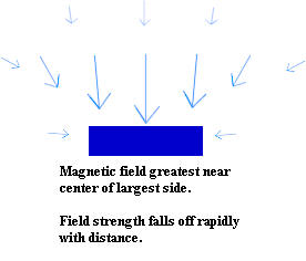
The field of the magnet is as shown in
the next figure. Note that the field drops rapidly as we move away from
the magnet, and that the field is strongest near the center of the largest face
of the magnet. To the right and left of the magnet, as drawn below, the
field is pretty weak and rapidly becomes insignificant as we move away from the
magnet.
Given these characteristics of the
force field:
- Should the path of the ball change
suddenly at a single instant or is the change in direction spread out over a
significant distance and time? Whichever your answer, why should it be
so?
- At what position along its path
would you expect the faster ball to be changing its direction most rapidly?
Which of the paths shown in the figure
below is more consistent with your previous answers? Why?
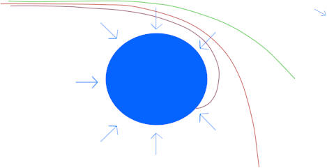
The figure below shows a hypothetical
circular disk magnet, which attracts steel objects equally around its entire
circumference, and always toward its center. It is not clearly indicated
in the figure but again this field is to be regarded as decreasing rapidly as we
move away from the disk.
[ Note: This is example
depicts a magnetic monopole, a magnet with just a 'north' or just a 'south' pole
without the opposite pole. No magnetic monopole has ever been observed in
nature (why a monopole has never been observed is unknown, and is one of the
great mysteries of physics). So nobody has ever created such an object and
we are now in the realm of imagination. ]
Three paths are shown below for a steel
ball rolled past this hypothetical circular magnet, from left to right..
- Which of the three balls had the
highest initial velocity and which the lowest?
- Would it be possible for a ball
having the right speed to go partway around the circle and end up moving to
the left away from the circular magnet?
- Would it be possible if the initial
velocity was just right for the ball to fall into a perfectly circular path
around the disk?
(b) NOT CURRENTLY
ASSIGNED: A fairly small arc of a circle is sketched on a
piece of paper and placed on a flat plane tilted in the x direction to simulate the
acceleration of gravity in that direction, with the x direction coinciding with the axis
of symmetry of the arc. The plane is tilted also in the y direction in such a way as to
just compensate for the frictional resistance to a ball rolling across it in that
direction. A curved-end ramp is used to give a steel ball a controlled initial speed and
direction, and the speed and direction necessary for the ball to maintain a path at a
(nearly) constant distance 'above' the arc are observed.
The tilt of the plane in the x direction can be
adjusted to mimic the relative strengths of the gravitational field at various distances
from the arc, and 'orbits' at these distances can be simulated.
Experiment 26. From a simulation we find that orbital
velocity is inversely proportional to the square root of orbital radius; potential energy
increase from one orbit to another is double the kinetic energy decrease so we have to
speed up to slow down.
Click here for instructions using the former DOS version of the program,
which is located under Simulations on the 'real' Physics I homepage. This
program should only be used if the program downloaded from the Sup Study ...
site does not work.
Instructions for program grav_field_simulation.exe for Experiment 26:
The program will be found at the Sup
Study ... site under Course Documents > Downloads > Physics I. Download and/or run it in order to see the buttons
and boxes described here:
The array of boxes and buttons at the right side of the screen
contains information about the planet, the satellite and the time scale of the simulation.
Planet mass is the mass of the planet in multiples
of the mass of the Earth. The default values assume that the planet is Earth, so the
default planet mass is 1. You can enter any planet mass you wish. For example the Moon has
a mass about 0.0123 times that of the Earth, the Sun has a mass which is about 340,000
times that of the Earth. If you wanted to simulate and orbit around the Sun or the Moon
you would enter 0.0123 or 340,000 in this box.
Planet radius is given in multiples of the radius
of the Earth. Since the default planet is Earth the planet radius has default value 1. If
you wanted to simulate the Moon you might enter 0.26, which represents the fact that the
Moon has a radius about 0.26 times that of the Earth. If you what and to simulate the Sun
you might enter 1100, since the Sun has a radius about 1100 times that of the Earth.
Time factor is the factor but which the simulation
is speed up. The default value of the time factor is 1,000, which means that everything
runs about 1000 times faster than actual. This means, for example, that a low-Earth orbit
will take place in about six seconds rather than the actual approximate time of 6,000
seconds.
Screen scale is the distance from the center of the
picture to the edges, in Earth radii. The default value is 3, which works well for low and
moderate Earth orbits. However if you are trying to investigate orbits which move further
than 3 Earth radii from the center of the planet you need to adjust the screen scale
accordingly or the satellite or projectile might not show up on the screen.
Initial distance is the distance of your satellite
or projectile from the center of the Earth. This distance is set to 1.02, which is around
the minimum distance at which it is possible to orbit at least a few times without
encountering significant atmosphere. You can set it for any distance you wish. [ Note that
this simulation ignores atmospheric drag and will work just fine for orbits inside the
atmosphere. In fact it ignores any sort of interference at all so orbits low enough to
encounter mountains will work just find here. Not only that, but this program implicitly
assumes that all the mass of the planet is concentrated at its center and even allows
orbits inside the surface of the planet. The only problem arises if you get very very
close to the center of the planet, in which case the simulation breaks down and spits the
satellite or projectile out at very high velocity in a straight line (which is just an
anomaly of the simulation and would not really happen in any circumstance). ]
Initial angular position is the angle in radians
made with the positive x axis (which is directed toward the right, as is standard for many
applications) by a line segment from the center of the planet to the initial position of
your satellite or projectile. Note that there are approximately six radians (actually 2
pi, closer to 6.28 radians) around a circle.
The impulse of the 'burn' is actually impulse per
kg. Recall that the impulse of a force acting on an object, which is the product F `dt of
the average force and time interval during which it acts, gives the change in the momentum
of the object. It follows that the impulse kg is in fact the change in the velocity of the
object. Note that we are here assuming that the 'burn' does not significantly change the
mass of the object; this is not always the case with actual satellites and certainly is
not the case with a rocket boosting a satellite into orbit. The default impulse is 8000,
which will give the satellite or projectile a velocity of 8000 m/s, a bit in excess of the
velocity required to achieve a circular low-Earth orbit.
To deliver an impulse you first choose the
magnitude of the impulse, then click on the Forward, Backward, To Right or To
Left button.
The direction of the initial impulse depends on the
goal of the simulation. If we wish to achieve a circular orbit then because of the
geometry of a circle (at every point the circle is perpendicular to the radial line from
the center to that point) the impulse must be at a right angle to the initial angular
position; otherwise circularity is in the first instant violated. Since a right angle is
1/4 of the angle around a circle, the right angle is 2 pi / 4 radians = pi / 2 radians, or
approximately 1.57 radians. On the other hand if we wish to shoot a projectile 'straight
up' from the surface of the Earth we must 'fire' it in the direction directly away from
the center of the planet, which means that we must 'fire' along the radial line from the
center to our starting point. This means that the initial direction must be the same as
the initial angular position.
Clock time is displayed as the simulation runs.
Clock time is the actual simulation time since the 'run' started.
Circle radius is the radius of a circular orbit you
might be trying to achieve, in Earth radii. If the number in this box is not zero
then when you click Run Simulation the program will place a red circle of this radius,
centered at the center of the planet, on the screen.
Realtime interval is the 'real world' time in
minutes since the simulation began.
Speed is the speed of the satellite or projectile
in meters/second.
The Run Simulation button is used to begin the
simulation. When the simulation is begun the planet will show in blue the center of the
screen and the satellite will show in white.
The first eight buttons in the rightmost column are
used to deliver an impulse to the satellite or projectile.
The top four buttons deliver the impulse forward,
i.e., in the direction of velocity of the object, or backward in the direction directly
opposite that of the object's velocity, or to the right (defined to be at a right angle to
the right as perceived by an individual facing the direction of motion) or to the left.
The default impulse is 0. The magnitude of the impulse
is chosen by clicking one of the next four buttons. Once clicked this
impulse is 'set' until another impulse button is clicked, so that it is possible with
successive clicks to deliver any reasonable chosen impulse.
The Pause Simulation button, as you might expect,
allows you to pause the simulation. There are two reasons you might want to do this.
One is to simply have a look at the numbers in the boxes, another might be to
change the numbers and restart the simulation without erasing the existing screen.
The Continue button will continue the program after
a pause; if you haven't changed anything in the boxes the program simply picks up where it
left off.
The Run (don't clear) button restarts the
simulation after a pause, without erasing the existing screen.
The 2d planet button will create a second planet
(e.g., the Moon), but first you have to go down to text boxes at the bottom of this column
(just above the Apply button) and enter the necessary information. The default message in
each box will tell you what you need to know, but those messages are repeated here.
Note that only the first word or two of each message actually shows in the box.
- The first of the two text boxes contains the message 'second planet
mass as multiple of Earth mass (Moon = .0123)', telling you to enter the mass of the
second planet, for example .0123 if you mean the Moon. Enter just the number with no
punctuation (except a decimal place if required) and no letters or words.
- The second box contains the message 'second planet dist as multiple
of Earth radius (Moon = 60.2)', meaning that you should enter the number 60.2 if you want
to simulate the Moon, or any appropriate number if you want to set up some other
situation.
Be sure you have the correct numerical information in these
boxes. If you don't the program is likely to crash.
After entering this information you can click on the 2d planet
button, which will give you a message telling you that the 2d planet has been created. If
the simulation is already running the second planet should appear, provided the screen
scale can accommodate it. If not, or if you wish to make other changes, you may change the
screen scale and any other information you wish then click on Run Simulation.
Suggestions for first-time use:
Without changing anything click on Run Simulation. You will see a
blue circle representing the Earth and a moving white dot representing the successive
positions of a satellite. The satellite completes its orbit 1000 times as fast as an
actual satellite, due to the default time factor.
While the simulation is running click on 'Impulse 100' then on
Forward and see what happens to the orbit.
Click on Forward a few more times and see what happens to the orbit.
Click on 'Impulse 1000' then on 'forward' and see what happens. Then
click on 'right' and on 'left' and see what happens.
Any time the simulation gets out of control you can started over by
clicking on Run Simulation. See if you can figure out the most efficient way to move from
the default orbit into a 'higher' circular orbit.
Do this:
- See how efficiently (i.e., in how few
clicks) you can get the satellite to the edge of the screen using 100 (kg
m/s) / kg impulses, starting from the default orbit.
Start the simulation over:
-
If you start from the basic orbit and supply a 1000 (kg
m/s) / kg impulse, in such a way as to maximize the KE change, what happens
to the maximum and minimum KE of the projectile?
-
If you supply a second 1000 (kg / s) / kg
impulse, in such a way as to maximize the KE change, what happens to the max
and min KE of the projectile?
-
If you supply a third 1000 (kg / s) / kg impulse,
in such a way as to maximize the KE change, what happens to the max and min
KE of the projectile?
-
What do you think would happen to the max and min KE if
you supplied a fourth 1000 (kg m/s) / kg impulse?
Change the initial impulse:
- Note that the default impulse of 8000, which gives the satellite an
initial velocity of 8000 m/s, gives an orbit which is not quite circular. Change the 8000
to 9000 and click the Run Simulation button to see how the orbit changes as a result of
the greater initial velocity. Then change the impulse to 7000 and click the Run Simulation
button to see what happens. Then see if you can find the initial velocity that gives you a
good circular orbit.
Achieve circular orbits at 1.5 and 2 Earth radii:
Put the satellite into a circular orbit and investigate:
- What immediate effect does a single impulse to the right or left have on the speed
of the satellite moving in a circular orbit?
'Shoot' a projectile 'straight up' from the
surface: To shoot 'straight up' you shoot straight out along a radial line (see direction
of the initial impulse in the description of the program above).
- First set the number in the Circle Radius box to 2.
- To position the projectile on the surface set Initial
Distance at 1, to place the projectile at 1 Earth radius from the center.
- Set Initial Angular Position to 1, which will place the
projectile at the 1-radian position.
- Set Direction of Initial Impulse also to 1, which will
'shoot' the projectile in the 1 radian direction. This will 'shoot' the projectile
straight out from the Earth, which from the perspective of an observer at that position
will appear to be 'straight up'.
- Reduce the Initial Impulse from its default
value of 8000 to 6000.
- Click on Run Simulation. See how far out from the
planet the projectile goes before 'falling back'.
- Repeat for Initial Angular Positions of 2, 3, 4, 5 and 6
radians, with initial impulses of 4000, 5000, 7000, 8000 and 9000. Be sure in every
case to set the Direction of Initial Impulse so that the projectile 'shoots' straight away
from the Earth.
- See which initial impulse gets the projectile closest to
the radius-2 red circle. Estimate the impulse you would need to exactly reach that
circle without 'overshooting' it and test your estimate.
The Experiment:
To start with you will determine the velocity required for a circular
orbit at a distance of 1.2 Earth radii.
Set Initial Distance at 1.2. Leave the remaining settings as they
are and click Run Simulation.
Determine from the shape of the resulting orbit whether the initial
velocity is too high or too low and change the number in the Initial Velocity box to a
value you believe will bring the orbit closer to a circular shape. The click Run
Simulation.
Repeat until you have achieved a good circular orbit and record the
velocity.
Now find the velocity with which a projectile would have to be 'shot'
from the surface of the Earth, ignoring air resistance, to get 'up' to the altitude of the
orbit you have just created.
- Pick a reasonable initial velocity.
- Position the initial angular position at 0 radians and make an
appropriate selection for the direction of the initial velocity (see the initial
introduction to the program under Suggestions for first-time use
above).
- Set the Time Factor to about 200 in order to give yourself time to judge
when the object has reached is maximum altitude.
- Pause the simulation before the object has much time to fall back to
Earth because if the projectile falls back to Earth then through to the center you might
like the result but it won't help you.
Repeat but change your initial angular position to 1 radian (and of
course change the initial direction of the 'shot' accordingly), and adjust your velocity
to get closer to your goal. Adjust the time of the simulation to allow the
projectile to stop moving outward and begin falling back. Continue changing the intial
angular position and your angular velocity until you manage to just reach the circular
orbit you created in the first part of the experiment.
Repeat this procedure for the orbital radius you have been
specifically assigned.
That is, determine the velocity necessary to maintain that orbit and the
velocity required to achieve the altitude of that orbit.
If you have not been assigned an orbital radius use 1.2 + .1 * (number
of letters in your first name).
Now achieve an elliptical orbit that just skims the surface of the
Earth.
Starting from a position at 2 Earth radii from the center, adjust your
initial velocity until you have an orbit that at its 'lowest' point just touches the
Earth's surface. Observe everything you can about the motion of the satellite in
this orbit, including the maximum velocity.
Analysis
For each radius you investigated determine, by setting centripetal
acceleration equal to gravitational acceleration, the 'actual' velocity for that circular
orbit.
Compare with the velocities you obtained.
According to your observations:
- How much KE per kg is required in your initial 'shot' to get to the
'altitude' of each orbit? How much does the PE of the projectile change as it
'climbs' to each orbit?
- What is the KE per kg in each orbit?
- By how much does the PE therefore change between the two circular orbits
you investigated?
- By how much does the KE change between the two circular orbits you
investigated?
- How are the PE and KE changes related?
According to theory:
- How much KE per kg is required in your initial 'shot' to get to the
'altitude' of each orbit? How much does the PE of the projectile change as it
'climbs' to each orbit?
- What is the KE per kg in each orbit?
- By how much does the PE therefore change between the two circular orbits
you investigated?
- By how much does the KE change between the two circular orbits you
investigated?
- How are the PE and KE changes related?
For the elliptical orbit, based on your observations:
- How does the velocity of the satellite at the 'initial' position 2 Earth
radii from the center compare to the velocity as it 'skims' the surface?
- What happens to the KE between the extreme furthest distance from center
and the closest approach to center?
- What happens to the PE between the extreme furthest distance from center
and the closest approach to center?
- Are your observations consistent with the conservation of energy?
For the elliptical orbit, based on theory:
- By how much should the KE of the satellite change from 'initial' position
2 Earth radii from the center and the point where it 'skims' the surface?
- What therefore should be the velocity of the object as it 'skims' the
surface, assuming that the initial velocity you gave it was accurate? How does this
velocity compare to the velocity you observed?
Speculate on what sorts of strategies are required to get a Space
Shuttle into a circular orbit at an 'altitude' of 400 km. Keep in mind that rocket
fuel doesn't carry enough energy to even get its own mass into orbit.
Speculate on what strategies are required to get a spacecraft to the
Moon, which is about 60 Earth radii away, and back. Note that you can if you wish
experiment with this situation by following the instructions for 2d Planet; just be
careful to set your original parameters so that the Moon is visible.
Instructions for DOS program (ignore if you have performed the Windows
version of this experiment)
We begin by determining the kinetic energy required
to get from the surface of the Earth, at 1 Earth radius from the center of the planet, to
1.2 Earth radii, then to 1.4 Earth radii, then to 1.6, 1.8 and 2 Earth radii.
- Ignoring air resistance, we will determine the
'vertical' velocity required to shoot an object of arbitrary mass m from the surface of
the Earth to various distances from the center of the Earth.
- The object will start out at the surface of the
Earth, which is 1 Earth radius from the center.
- You may choose to position the object at any angular
position and 'shoot' the object in the direction defined by the same angle, so that it
will start out moving directly away from the Earth and all of its KE will be dissipated in
the process of reaching its maximum 'altitude'.
- The velocities you will need to use are generally in
the range from 1,000 to 12,000 m/s. Select a velocity from this range and see how far the
object ends up from the center of the Earth.
Your goal is to end up at a distance of 1.2 Earth
radii from the center. Find the velocity that gets you as close as possible to that
distance.
- Repeat, this time determining the velocity required
to get to a distance of 1.4 Earth radii from the center.
- The object went twice as 'high' as in the first
trial. Did it take twice as much velocity, more than twice as much or less than twice as
much?
- Assuming that the mass of the object is m, determine
the kinetic energies at the surface of the Earth required to achieve each distance.
- Did it take twice as much KE, more than twice as
much or less than twice as much, as in the first trial?
- Repeat for distances of 1.6, 1.8 and 2.0 Earth radii
from center. Give careful attention to the velocity changes required, and especially to
the KE changes required.
- Make a table of velocity at surface and KE at
surface vs. max. distance from Earth center.
- Make a graph of velocity at surface vs. max.
distance from Earth center.
- Make a graph of KE at surface vs. max. distance from
Earth center.
- How much KE is necessary to move an additional .2
Earth radii from the center, starting at the surface of the Earth? How much is required
starting at 1.2 Earth radii from the center? How much is required at 1.4, 1.6, 1.8 and 2.0
Earth radii from the center?
- How can each of these kinetic energies be found on
the graph of KE vs. max. distance from center?
- How much KE would be required at a distance of 1.4
Earth radii from center to reach 1.8 Earth radii from center? How could this KE be found
the graph of KE vs. max. distance from center?
- How much KE would be gained by an object, initially
at rest at a distance of 2.0 Earth radii from the center, if it 'fell' to a distance of
1.6 Earth radii from the center? Explain how the answer to this question tells you the
difference between the gravitational PE of the object at 2.0 Earth radii and at 1.6 Earth
radii from center. At which point is the gravitational PE higher? How does this situation
illustrate the conservation of energy?
We now determine the velocity required for a
circular orbit and orbital radii of 1, 1.2, 1.4, 1.6, 1.8 and 2 Earth radii.
- To achieve a circular orbit, the velocity of the
satellite must at every point be perpendicular to the radial line from the center of the
planet to the satellite. This is a simple consequence of the geometry of a circle, for
which attention line must always be perpendicular to the radial line.
- The only way to achieve a circular orbit is
therefore to give the satellite a velocity which is at a right angle (i.e., an angle of
about 1.57 radians) to its angular position. This could be done with an angular position
of, say, 1 radian and a velocity at either 2.57 radians or -.57 radians, either of which
would be perpendicular to the radial line. It is probably easiest to simply start the
satellite and angular position of 0 with a velocity in the direction 1.57 radians.
- Begin at an orbital distance 1 Earth radius, and
determine the velocity necessary to give you a circular orbit of the planet. If your
chosen velocity is too low, the satellite will appear to orbit in an elliptical path
inside the planet (the simulation is unaware of the disadvantages of this sort of orbit).
If your chosen velocity is too high, you will experience and elliptical orbit outside the
surface of the planet (much more convenient, though in reality air resistance would be a
problem, not to mention things like mountains, people and tall buildings, all of which the
simulation is completely unaware).
- Repeat for orbital radii of 1.2, 1.4, 1.6, 1.8 and
2.0 Earth radii.
- For each orbital radius, determine the KE of a
satellite of mass m at this radius.
- Place these values of the KE in a table.
- By how much does the KE of a satellite of mass m
change between orbital radii of 1 and 1.2 Earth radii? What is the change between 1.2 and
1.4 Earth radii, between 1.4 and 1.6 Earth radii, between 1.6 and 1.8 Earth radii and
between 1.8 and 2.0 Earth radii? Are the KE changes positive or negative?
- What is the PE change from 1.0 to 1.2 Earth radii?
Is the PE change positive or negative? What therefore is the net change in energy between
1.0 and 1.2 Earth radii? Is the net change positive or negative?
- If a satellite is to change its orbit from 1.0 to
1.2 Earth radii, what must happen to its altitude and its speed? How then should it fire
its thrusters?
Consider the proportionalities involved in energies
and velocities.
- Sketch a graph of kinetic energy vs. orbital radius,
for orbital radii from 1.0 to 2.0 Earth radii.
- It is clear that the kinetic energy decreases with
orbital radius. We wish to determine whether there is a proportionality between the
kinetic energy and orbital radius. We will test the proportionalities KE = k / r, Ke = k /
r^2 and KE = k / `sqrt(r) to determine whether KE is might or might not be inversely
proportional to r, to `sqrt(r) or to r^2.
- Sketch graphs of KE vs. 1/r, KE vs. 1/r^2 and KE vs.
1/`sqrt(r) and determine if one of these graphs is linear. If so, then it indicates the
appropriate proportionality and k is the slope of the graph.
- Since KE is proportional to v^2, then what should be
the proportionality between v and r? (The proportionality should be of the form v = k /
r^p for some value of p; so what is p?)
We now consider the behavior of the satellite in an
elliptical orbit.
- Create an elliptical orbit which moves to within 1
Earth radius from the center at its closest point, and which has a maximum distance of 2
Earth radii from the center.
- Does the satellite move faster near the planet or
far from the planet?
- As best you can determine the ratio between the
speed of the satellite at its maximum distance to its speed at the minimum distance?
- Speculate on what the ratio would be between the
speed of the satellite at maximum distance and at minimum distance is the maximum distance
was 3 times the minimum.