From all the evidence you have gathered, what is the wavelength of the light from the laser and what is the grid spacing of the diffraction grating?
Explain in detail what's going on when you measure the beats resulting from the computer-generated sound and the rod. How accurately do you think you could measure the frequency of the rod's vibration?
Find the propagation velocity of the wave you measured, assuming rod length 152 cm.
Using v = sqrt(Y / rho), where rho is the mass density of aluminum (2700 kg / m^3), determine Y for aluminum.
Two discrete light sources emit waves in all directions, as depicted below.
A large number of sources will each behave in the same manner.
In the figure below we depict waves emitted in phase at 15 points, each wave running along one a downward-sloping lines. All these lines are parallel. The upward-sloping lines are perpendicular to the waves.
We can imagine that the lines indicating the directions of the waves are not quite parallel but in fact meet at a distant point. All points of the perpendicular lines lie at equal distance from the distant point where the waves meet.
The same figure, in closeup, is shown below. We see how the peak of each waves aligns with the peak of every other wave so that the peaks will reinforce at the distant meeting point.
If the figure below represents selected light rays emitted by a number of in-phase sources (e.g., by a diffraction grating). The selected rays are emitted at the same angle with the line connecting the sources.
If the distance between
adjacent upward sloping lines is 2 wavelengths, then
If the distance between adjacent upward sloping
lines is 1.07 wavelengths then
Answer the same questions for if the path difference is 1.19 wavelengths, and if the path difference is 1.01 wavelengths.
Consider first the case where the spacing is 2 wavelengths. The figure below shows the waves as they would appear if every wave is emitted as a sine what with phase angle 0. It should be clear that the wave emitted by each source lags the one emitted by the source below it by 2 wavelengths, and the one two sources below by 4 wavelengths, etc., so that the peaks of each wave will arrive at a distant detector in phase with the peaks of every other.
A closeup of the same figure is shown below. Note how once again each peak of every wave aligns with the peaks of the other waves.
For path difference = 1.07 wavelengths we have the figure below. Note how the peaks of the wave emanating from source #13 appear to align with the valleys emanating form source #6
The closeup in the figure below shows how the peaks of waves #1, 2, 3, ..., 8 each shift a bit to the left of the preceding. For every wave there is another whose valleys very nearly align with its peaks.
For example wave #2 is 1.07 wavelengths behind #1, #3 is 2.14 wavelengths behind #1, #4 is 3.21 wavelengths behind #1, #5 is 4.28 wavelengths behind #1, #6 is 5.35 wavelengths behind #1, #7 is 6.42 wavelengths behind #1 and #8 is 7.49 wavelengths behind #1. This causes phase shifts of .07, .14, .21, .28, .35, .42, .49 wavelengths with respect to #1.
The pattern continues with shifts of .56, .63, .70, .77, .84, .91 and .98 wavelengths.
Every wave can be matched with another that very nearly cancels it. If the figure was extended to show hundreds or thousands of sources, it would be possible to match up each wave with another that exactly cancels it.
For path difference = 1.19 wavelengths we can again see the near-cancellation of each wave by some other wave. Again we see that if there are a large number of sources each wave could be matched up with another that exactly cancels it.
For path diff = 1.5 wavelengths each wave exactly cancels the next.
For path diff = 2.5 wavelengths we again see the perfect cancellation of each wave with the next.
In the figure below the path difference is 1.25 wavelengths. An accurate picture is depicted just to the right of that figure. We see that the peaks of one wave align imperfectly with either the peaks or the valleys of the other.
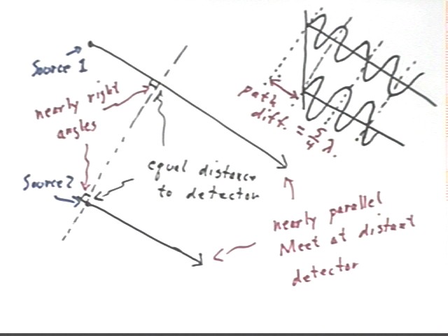
The lines along which the wave travels are nearly parallel, meeting at a very distance detector.
The dotted lines are considered to be at equal distances from the distant detector, so they are at nearly right angles with the directions of the waves.
The path difference, i.e., the extra distance traveled by the wave from source 1, is therefore the distance from that source to the dotted line.
In the small picture in the upper right corner of the figure the dotted lines are equally spaced, each spacing equal to the path difference. The wave is drawn so that the path difference is equal to 5/4 of the wavelength.
If we 'straighten out' the above picture by viewing it at the appropriate angle it will look something like the figure below. In this figure we have inserted vertical lines at quarter-wavelength intervals.
The next figure is a 'closeup' of the two waves between the first and third vertical line. Be sure you see how this picture is correlated with the one above.
At the position of the second vertical line (counting from the left) the top wave is at its peak and the bottom wave is at its equilibrium point. At this point the sum of the two waves will therefore result in a vertical displacement equal to the amplitude of the top wave.
At the position of the third vertical line the bottom wave it at its peak and the top wave at equilibrium, so that the sum of the two waves will have vertical displacement equal to that of the bottom wave.
Between the second and third line the top wave decreases while the bottom wave increases. The rate of decrease of the first wave is at first less than the rate of increase of the second, so that the sum of the two waves must reach a maximum which is greater than the sum at the position of the second line.
Because of the symmetry of the situation the maximum will occur exactly halfway between the second and third vertical line.
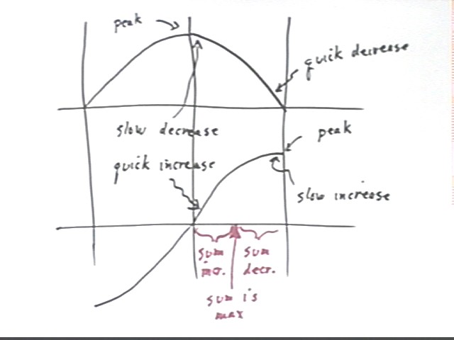
The figure below illustrates the sum of the two waves, depicted by the graph lying between the top and bottom waves. Be sure you see how between the second and third lines this sum wave has the characteristics described above. Then verify for yourself that over the next few quarter-cycles the sum wave behaves as we would predict.
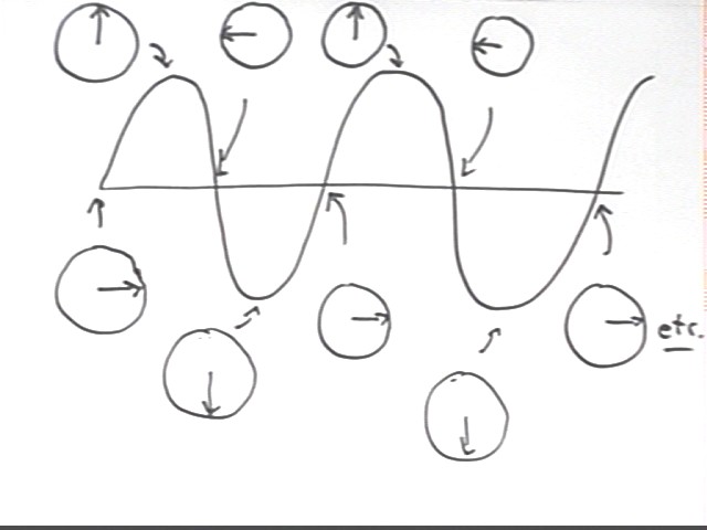
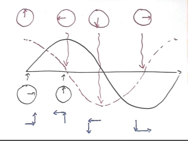
The first wave is depicted below. We consider the wave to be moving toward the left. Recalling the circular model of SHM we easily see how the circles correspond to the motion.
For example at the leftmost point of the graph the string is at its equilibrium position. The circle below the leftmost point of the graph shows a reference-circle depiction of SHM at the equilibrium position and moving upward.
The first 'peak' of the graph corresponds to a reference-circle picture of the maximum upward displacement in SHM.
The reference-circle picture for the next equilibrium position represents SHM at equilibrium and moving downward.
The reference-circle picture for the first 'valley' corresponds to the maximum negative displacement.
As the cycle ends we see that the reference-circle picture is back to the original configuration, and that the series of reference-circle pictures repeats.
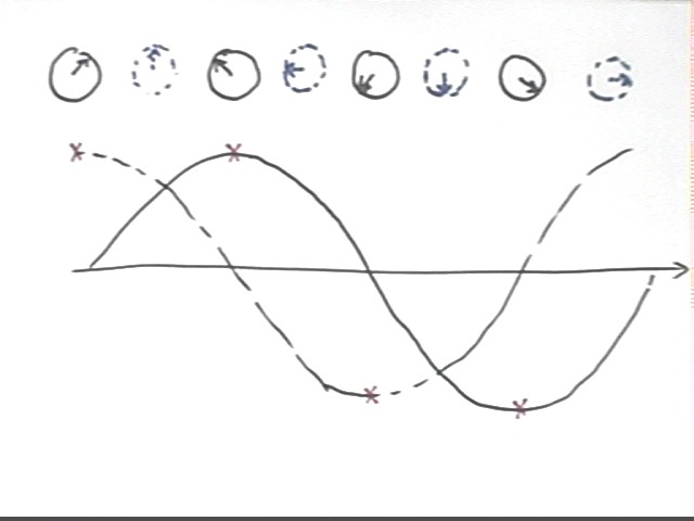
In the figure below we consider two waves which are 1/4 cycle, or 90 degrees, out of phase.
The reference-circle pictures above the graph correspond to the dotted-line graph, and those below to the solid-line graph. Be sure you see why the reference-circle pictures are as shown.
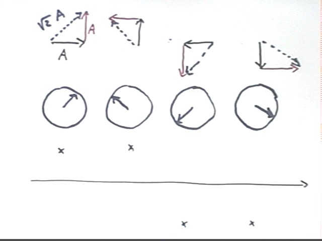
The vector diagrams at the bottom of the figure represent the two reference-circle vectors at the corresponding points of the graph. We note that since the waves are 90 deg out of phase the vectors in each picture are at right angles.
We again show the vectors in the figure below. The first pair, corresponding to the leftmost point on the graph, is labelled to show that the amplitudes of the two waves (which for this example we consider to be equal) correspond to the magnitudes of the two vectors.
The hypotenuse is the resultant, corresponding to the sum of the two vectors. You should verify that the hypotenuse should have magnitude sqrt(2) * A.
Directly beneath the vector diagram is a reference circle indicating the resultant of the two vectors.
Reference circles are sketched for all four diagrams. The first two indicate positive displacements from equilibrium, the second two negative displacements.
The horizontal axis beneath the sketch represents the equilibrium position of the string. The x beneath each circle represents the vertical displacement at the corresponding position on the wave:
The figure below duplicates the circles in the figure above and adds the original sketch of the two waves. The four x's from the preceding figure are included. The dotted circles clearly fit the sequence of the four solid circles and represent the reference circles at in-between positions.