Calculus II
Class Notes, 1/15/99
We begin with the last example from the preceding
class:
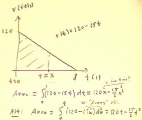
To obtain the distance function as
an area integral of the velocity function, we can
find the position change from clock time t = 0 to the
variable clock time t = x.
- The position change is indicated by
the area of the shaded region of the graph below.
- This area is the integral from
t = 0 to t = x of the velocity function,
as indicated below.
- If we complete the integration we find that the
distance is s(x) = 120 x - 15/2 x^2.
It doesn't make a lot of sense to use x for
a clock time; we use w as a dummy variable of
integration so we can use t as a limit on the integral,
and obtain s(t) = 120 t - 15/2 t^2 as our distance function..
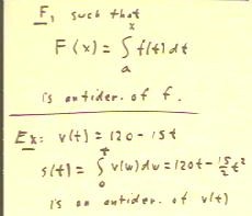
We see that the distance function obtained
by this integration is an antiderivative of the velocity function.
More generally, the Second Fundamental
Theorem of Calculus tells us that such a process will always give us an
antiderivative function. The statement of this theorem goes something like the
following:
- A function F such that F(x) is the definite
integral of f(t), between some fixed limit a
and the variable limit x, must be an antiderivative of
the function f.
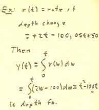
As another example of the application of this
Theorem, we recall that if r(t) is the rate at which the depth of
a fluid in a cylinder changes, then the depth
vs. time function is an antiderivative of this rate function.
- In the example below we see that when we integrate
the rate function between t = 0 and t, using the dummy
variable w as our variable of integration, we obtain the antiderivative y(t)
= t^2 - 100 t.
- This antiderivative is a depth
function.
- This depth function has the characteristic that y(0)
= 0, so that depth is measured from the t = 0 point.
- If we wish to change the depth function so that depth
is measured from a different point, we need
only add the appropriate constant.
- Adding a constant does not change
the derivative of the depth function, so the rate function will
remain unchanged.
In the example we find an antiderivative of the
function x^3 sin(x^4), using inspection and our knowledge of the chain rule.
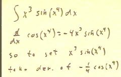
It is not always easy to find an antiderivative by inspection.
In the example below we use a more formal means of finding the
antiderivative, called substitution.
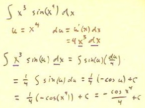
- Knowing that sin(x^4) is a composite function, with 'inner
function' u(x) = x^4, we set u(x) = x^4 and write down its differential
du = 4 x^3 dx.
- We can then write sin(x^4) as sin(u), which is a simple
function of u and no longer looks like a composite function.
- We then note that the remaining factors in the integral are x^3
dx, which appears in our expression for du.
- In fact we easily see that x^3 dx = du / 4.
- We can therefore rewrite the expression under the integral as sin(u) du / 4,
which we proceed to integrate in the next step.
- Our antiderivative is 1/4 (-cos(u)) + c.
- We now substitute x^4 back into the expression for u,
obtaining antiderivative - cos(x^4) / 4 + c.
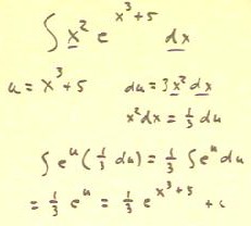
We apply the same strategy to the integral below.
- We identify x^3 + 5 as the 'inner function' of a
composite and write u = x^3 + 5.
- We write down the differential du, and solve for the
variable part x^2 dx of the resulting equality.
- Noting that the expression under the integral consists of x^2 dx = 1/3 du and
e^(x^3 + 5) = e^u, we rewrite the integral and perform
the integration.
- We finally substitute u(x) = x^3 + 5 back into the resulting
antiderivative and belatedly add our integration constant c (it should have appeared one
step earlier).
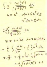
The example below is a bit more complex.
- As before we let u = x^6 stand for the 'inner function' in a composite,
while noting with some discomfort that x^6 appears in this role in more
than one function (we might even notice that one appearance is as the innermost
function of a composite of a composite).
- We proceed in the usual manner and determine that x^5 dx = 1/6 du.
- We rewrite the integral in terms of u and du.
We note that we still have an integral involving the composite function `sqrt(sin(u)).
In fact we are little bit apprehensive about the fact that this function appears in
reciprocal form, so that we still have a composite of a composite.
- We let w = sin(u), the innermost function of our
existing composite.
- Rewrite down the differential dw and note with a glimmer of optimism
that it involves the expression cos(u) du, which in fact appears in our
integral.
- Our glimmer of optimism turns to outright joy as we rewrite our integral in terms of w
and dw, and we recognize that we can now find an antiderivative.
- We proceed to find an antiderivative, 1/3 w^(1/2), and substitute
w = sin(u) into this expression, then substitute u = x^6 into
the resulting expression to obtain our final antiderivative,
being assured to add the integration constant c at every step.
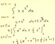
If we have limits on a definite integral, we can deal
with them in one of two ways:
- We could first find the antiderivative 1/2 e^(x^2) and substitute
the limits into this expression in the usual manner, obtaining 1/2 e^(3^2) - 1/2
e^(0^2) = 1/2 (e^9 - 1).
- We could alternatively transform the integral into the
integral of e^u du, with u = x^2, and simultaneously transform
the limits on our integral into limits on the new variable of
integration u.
- If the limits on the variable x are 0 and 3, the limits on the variable
u = x^2 will then clearly be 0 and 9.
As shown below we obtain the same result either way.