f(x) Notation; The Generalized Modeling
Process
Introduction to function notation
The function notation f(x) allows us to refer to function
behaviors y characteristics without reference to a specific function.
For example, if we wish to say that the y intercept of a
function occurs when the variable x is equal to 0, we could refer to a specific example as
follows:
If we have a function, for example y = 3x^2 + 2x - 4, its
y intercept occurs when x = 0. This occurs when y = 3(0^2) + 2(0) - 4 = -4. Thus the y
intercept occurs at (0,-4).
If we understand that f(x) stands for the expression 3x^2
+ 2x - 4, so say for example f(7), where the x has been replaced by the 7, stands for the
expression 3(7^2) + 2(7) - 4, we can make the same statement more generally for all
functions by saying
If we have a function y = f(x), its y intercept occurs
when x = 0. This occurs when y = f(0). Thus the y intercept occurs at (0, f(0)).
This function notation has a great number of advantages,
and will be used commonly throughout this course. The purpose of this exercise is to
become familiar with the nature of the notation.
Examples of the f(x) notation
Example 1: f(x) = 3x^2 + 2x - 4
As the first example let us suppose replace f(x) stands
for the previous expression 3x^2 + 2x - 4. So we have defined the function
f(x) = 3x^2 + 2x - 4.
As we saw before, when we wrote the expression f(7), we
replaced the x in the original expression with the number 7. We therefore replace every
instance of x by 7 to obtain
f(7) = 3(7^2) + 2(7) - 4.
We can of course evaluate the expression to obtain f(7) =
157.
You should verify for yourself that f(1) = 1, f(2) = 12,
f(3) = 29, and f(4) = 52.
Replacing the variable by an algebraic expression
When we replace x, we need not replace it by a number. We
can for example obtain an expression like f(x-5). For this specific function, we have
f(x-5) = 3(x-5)^2 + 2(x-5) - 4.
This expression can be simplified as follows:
f(x-5) =
3(x-5)^2 + 2(x-5) - 4 =
<as above>
3 [(x-5)(x-5)] + 2(x-5) - 4 = ` <expressing
(x-5)^2 as [ (x-5)(x-5) ]>
3 [x(x-5) - 5(x-5)] + 2(x-5) - 4 =
<applying the distributive law to
[(x-5)(x-5)]>
3[x^2-5x - 5x+25] + 2x-10 - 4 =
<applying the distributive law again>
3[x^2 - 10x + 25] + 2x-10 - 4 =
<should be obvious; be sure -
sign distributes>
3x^2 - 30x + 75 + 2x-10 - 4 =
<distribute the 3>
3x^2 - 28x + 71.
The difference between f(x-5) and f(x) - 5
We can compare the results of this substitution with the
expression f(x) - 5. We don't substitute the 5 anywhere, since it doesn't replace anything
in the original expression f(x). It is just tacked on to the end.
f(x)-5 =
(3x^2 + 2x - 4) - 5 =
<substituting the expression
for f(x)>
3x^2 + 2x - 9.
<should be obvious>
We can compare these results with those obtained from the
expression -5 f(x), where again the -5 is not part of any substitution:
-5 f(x)=
-5 (3x^2 + 2x - 4)=
<substituting the expression
for f(x)>
-15 x^2 - 10x + 20.
<using the distributive law>
Substituting -b/(2a) for the variable in a
quadratic
Suppose that we substitute for x the coordinate of the
vertex of the quadratic function. We obtain y = f(-b/(2a)). We therefore write
y = f(-b/(2a)) = 3(-b/(2a))^2 + 2(-b/(2a)) - 4.
This expression can be expanded and simplified, though the
algebra is somewhat messy:
y = f(-b/(2a)) =
3(-b/(2a))^2 + 2(-b/(2a)) - 4 =
3( b^2 / (4a^2) ) - 2b / 2a - 4 =
3/4 (b/a) ^2 - b/a - 4.
The precise form of the simplified expression depends upon
what we're using the expression to understand. In this case we simplified the expression
in such a way as to show that f(-b/(2a)) can be seen as a quadratic with variable (b/a).
We also note that if f(x) represents the general quadratic
function f(x) = ax^2 + bx + c, then -b/(2a) represents the x coordinate of the vertex of
the parabola. In this case f(-b/2a) will be represented as follows:
y = f(-b/(2a)) = a (-b/(2a) )^2 + b(-b/(2a)) + c.
We might wish to simplify this expression:
y = f(-b/(2a)) =
<substituting -b/(2a) for x>
a (-b/(2a) )^2 + b(-b/(2a)) + c = <substituting
-b/(2a) for x>
a (b^2 / (4a^2) ) - b^2 /(2a) + c =
<simplifying individual
terms>
b^2 / (4a) - b^2 / (2a) + c =
<simplifying individual
terms>
b^2 / (4a) - 2 b^2 / (4a) + c =
<common denominator for first
two terms>
-b^2 / (4a) + c.
<adding terms>
Then we could write
yVertex = f(xVertex), so
<evaluate function at xVertex
to get yVertex>
yVertex = f(-b/(2a)) from which
<xVertex is -b/(2a) from quad
formula>
yVertex = -b^2 / (4a) + c.
<f(-b/(2a)) from before>
Note that the purpose here is not to learn the algebra
used in the above steps, but to look at examples of the use of the function notation.
However the algebra does provide a useful review of some common and important procedures.
You should write out the algebra steps in standard mathematical notation and ask questions
about anything you don't understand.
1. Of course you know, or at least suspect, that
your function models won't always be quadratic. Obtain the indicated expressions for the following
functions, none of which are quadratic:
Where f(x) = x^3, find f(-2), f(2), f(-a), f(a), f(x-4)
and f(x) - 4.
Where f(x) = 2^x, find f(-2), f(2), f(-a), f(a), f(x+3)
and f(x) + 3.
2. You should also be aware that we can use letters
for our functions other than f. We can denote a function by the notation g(x), h(x), y(x),
Q(x), Z(x), changeRate(x), investmentValue(x), or whatever. Each of these expressions
indicates a quantity that varies with x. And we don't have to use the letter x to stand
for the variable. We can have expressions like A(t), V(z),
accumulatedTotal(investmentStrategy), or gradeEarned(timeDevoted). In each case we say
that the quantity in the parentheses is the variable.
Obtain expressions for the following:
Where value(t) = $1000 (1.07)^t
value(0)
value(1)
value(2)
value(t+3)
value(t+3)/value(t).
Where illumination(distance) = 50 / distance^2:
illumination(1)
illumination(2)
illumination(3)
illumination(distance)/illumination(2*distance).
We can generalize the modeling process
by referring to a general function denoted by y = f(x) instead of the specific quadratic
function y = a t^2 + b t + c, or an even more specific function like y = .01 t^2 - 2 t +
100.
Examples of different forms include,
among many others:
y = a x^p with two parameters, a and
p
y = A * 2 ^ (kx) + c with three
parameters A, k and c
y = A x^p e^(kx) with three
parameters A, p and k
y = A sin(kx + `theta0) + c with
four parameters A, k, `theta0 and c.
In each case, when we substitute the
coordinates (x,y) of a data point we obtain an equation for the parameters.
In the modeling process, we often find
the parameters of our function model by solving a system of equations.
In the example of the quadratic
model the system consisted of linear equations.
When we substitute parameters into
the form we have chosen, we obtain a system of equations which might or might not be
linear.
We then solve the system to evaluate
the parameters.
We substitute the parameters into
the form of our function; our result can be represented by y = f(x).
Two of the main questions we can ask
about the function or its graph involve finding y for a given x, or x for a given y.
What follows is a modification of the
original summary of the modeling process, representing the process more generally.
Steps that have been modified are
marked with a double asterisk (**).
**
Substitute parameters
For a quadratic model we have solved for the
parameters a, b and c of the quadratic function y = f(x) = ax^2 + bx + c. We
substitute the parameters to get the specific function, e.g., f(x) = .01 t^2 - 2t + 100.
For an exponential model we would have the
parameters A, b and c of the exponential function y = f(x) = A b^x + c and
we would substitute them to get the specific function, e.g., f(x) = 100 (1.10)^x + 500.
For a linear model we would have the parameters m
and b of the linear function y = f(x) = mx + b, which we would substitute to
get the specific function, e.g., f(x) = 2x + 7.
For a pth-power model we would have the parameters A,
h and c, which we would substitute to get the specific function, e.g., f(x) = A [
(x-h) ] ^ p + c.
For any function model, we obtain a model which can be
represented as
y = f(x)
** Graph the
model
We graph the model with the data points in order to
compare the model with our data.

Linear, quadratic, exponential, and positive- and
negative-power functions each have their own typical shape, which differs from the shape
of any of the other families. Only quadratic functions have parabolas as graphs. An
exponential or negative-power function will have an asymptote at some horizontal line
(i.e., it will approach the horizontal line more and more closely without ever actually
reaching it). A negative-power function will also have a vertical asymptote.
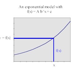
The exponential model has a graph with a horizontal
asymptote:

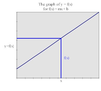
A linear model has a straight-line graph with slope m and
y=intercept b:

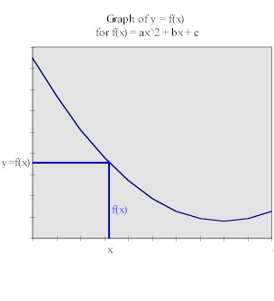
The quadratic model has a parabolic shape:

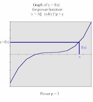
There are many different power functions, depending on the
power p. The power p=3 function has a point where its curvature changes from
downward to upward:

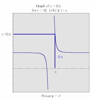
The power p=-3 function has both vertical and horizontal
asymptotes:

Any of these shapes can be uniformly stretched in the
vertical or horizontal direction or shifted vertically or horizontally. However, it is not
possible to shift and stretch the graph of, say, an exponential function into that of a
quadratic function, or a power p=3 function into a power p = -3 function. Each type of
function has its own family of graphs, and there is no overlap between families.
Quantify the comparison
Average of deviations = 2.43
** Pose
and answer questions
We ask of our model questions like
At what time t is the depth equal to 25 centimeters?
What is the depth y at time t = 48 seconds?
For how long is the depth y between 25 and 55 centimeters?
What is the range of depths y between t = 10 seconds and t
= 65 seconds?
At what distance x is the illumination y equal to 35
watts/square meter?
What is the illumination y at distance x = 22 meters?
For what distance range is the illumination y between 10
watts/square meter and 50 watts/square meter?
What illumination range will we experience between
distances x = 12 meters and x = 19 meters?
All these questions can be answered by using answers to
the following two questions:
Solve y = f(x) for y, given x.
Solve y = f(x) for x, given y.
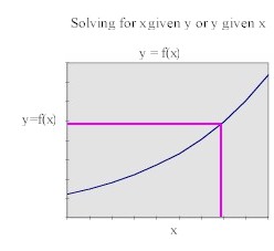
Approximate answers to these questions can be found from
the graph of the function model:
link to graphical solution ....
To find y from x we locate the specific value of x on the
x axis and see how far above or below the axis we have to go to reach the graph. This
distance is our value y = f(x), which can also be found on the y axis by moving
horizontally from the graph point to the axis.
To find x from y we simply reverse the process, locate the
specific value of y on the y axis and moving horizontally to the corresponding graph
point. The x coordinate of this point is found by moving vertically to the x axis.
** Substitute parameters
y = f(x)
** Graph the model

Quantify the comparison
Average of deviations = 2.43
** Pose and answer questions
Solve y = f(x) for y, given x.
Solve y = f(x) for x, given y.

3. Sketch a reasonable graph of y = f(x), if
it is known that f(2) = 80, f(5) = 40 and f(10) = 25.
Use your graph to estimate the following:
The value of x for which f(x) = 60.
The value f(7).
The difference between f(7) and f(9).
The difference in x values between the points where
f(x) = 70 and where f(x) = 30.
4. If a temperature vs. clock time function
is given by y = temperature = T(t), then what is the symbolic
expression for each of the following:
The temperature at time t = 3.
The temperature at time t = 5.
The change in temperature between t = 3 and t = 5.
The average of the temperatures at t = 3 and t = 5.
What equation would we solve to find the clock time
when the model predicts a temperature of 150?
How would we go about finding the length of time
required for the temperature to fall from 80 to 30?
5. Questions about your depth vs. time model
For your model of depth vs. time, based on in-class
measurements, answer the following questions and give detailed reasons for your answers as
well as sketches. Use the f(x) notation at every opportunity as you give and reason
out your answers:
For how long was the depth between 34 and 47 centimeters?
By how much did the depth change between t = 23 seconds
and t = 34 seconds?
On the average, how many seconds did it take for the depth
to change by 1 centimeter between t = 23 seconds and t = 34 seconds?
On the average, how by many centimeters did the depth
change per second between t = 23 seconds and t = 34 seconds?
6. A
hypothetical depth vs. time model based on three points, none of which are actual data
points
Sketch a graph of the following depth vs. time data:
( 0 sec, 96 cm)
(10 sec, 89 cm)
(20 sec, 68 cm)
(30 sec, 65 cm)
(40 sec, 48 cm)
(50 sec, 49 cm)
(60 sec, 36 cm)
(70 sec, 41 cm)
These data were obviously taken by someone with either bad
instruments or a high degree of incompetence. However, on the average they might well give
a good quadratic model.
Sketch the data and sketch a smooth curve that
doesn't touch any data points but comes as close as possible to the data points,
on the average. Your curve will go pretty much through the middle of the data set.
Pick three points on this curve, approximately equally
spaced in the y direction, and use them as a basis for constructing a function model.
Determine the average deviation for your model, and graph
your function.
How close is your model to the curve you sketched earlier?
How well does your function seem to model the data?
