NOTE: This document is probably redundant with the preceding document, the 12/08/98 document entitles 'Review I'.
The following review topics include questions that, along with minor variations on some questions, will be included in the problem bank for the final exam. Other questions not on this list will also be included, as will all questions from the problem banks for the two tests.
The review will consist of solutions to these questions and problems.
These questions and problems are classified as follows: The Modeling Process Equation Solving Properties of Functions
This document contains outlines of answers for the last two sections. The first section has been omitted from this document, and can be seen in the preceding set of class notes.
1. Solving Linear Equations
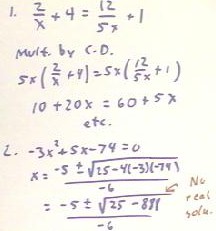
The solution of the first equation is straightforward. Simply use the distributive law of multiplication over addition, simplify both sides, and proceed in the accustomed manner. The solution is x = -19/12.
The second equation has denominators. The first thing we usually do we have equation with denominators should be to multiply the equation by a common denominator, carefully making note of the fact that the equation is not defined for those values that make a common denominator zero.
The solution of the second equation is shown below. We multiply by the common denominator 5 x, noting that the equation is not defined for x = 0. After using the distributive law and simplifying both sides, we can proceed in the accustomed manner.
2. Solving Quadratic Equations
The first equation is easily solved using the quadratic formula. The second equation is solved in the preceding figure; we note that because of the negative quantity under the square root we do not obtain a real solution. The solutions are x = -1.345207879 and x = 3.345207879.
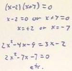
The third equation is easily solved, as in the figure below, by noting that the product of two factors can be 0 only if at least one of the factors is zero. In this case our solutions occur when x-2 = 0 or when x + 7 = 0; our solutions are therefore x = 2 and x = -7.
The fourth equation is easily solved by noting that we have only the x^2, x and constant terms of a quadratic equation. We put the equation into the standard form by subtracting 3x - 2 from both sides. The rest of the solution is straightforward, using the quadratic formula.
We use the same strategy on the fifth equation, adding 5x^2 to both sides. Our solutions are x = 4.959871174 and x = -7.459871174.
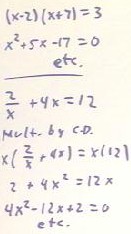
We might be tempted to solve the sixth equation by the same method we used in the third, but this would not work, since our solution of the third equation depended on the right-hand side being zero. To solve this equation, we must multiply the binomials and put the equation into the standard form of a quadratic. We then apply the quadratic formula, as usual, obtaining solutoins x = -7.321825380 and x = 2.321825380.
We solve the sixth equation by multiplying every term by the denominator x. After applying the distributive law we see that we have a quadratic equation, and put it into standard form. We then proceed as usual. We obtain the solutions
x = 2.822875655 and x = 0.17712434443. Solving Equations with Denominators
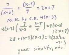
We solve the first equation by multiplying both sides by the common denominator 4 (x-3). After applying the distributive law we find that we have a quadratic equation. We will proceed to simplify both sides of this equation, then we will put the equation in the standard form of the quadratic and apply the quadratic formula. Our solutions are x = -5.201973235 and x = 3.487687521
We do not solve the second equation here, though we note that the common denominator is 10 (x + 3). This equation will, after simplification, give us a linear equation which we can easily solve, obtaining x = 31/3.
4. Solving Equation x^p = c
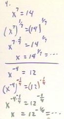
We solve the first equation by taking the 1/7 power of both sides, as in the first figure below. We evaluate 14 ^ (1/7) using a calculator, obtaining 1.457916249.
We solve the second equation by taking the -1/4 power of both sides, as shown below. We evaluate our final result using the calculator to get x = +- 0.5372849665.
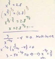
The third equation is solved by taking the 7/3 power of both sides, as shown in the second figure below. As usual the final result will be evaluated with the aid of the calculator to obtain x = 11.05016469.
The equation x^(-5/8) = 43 gives us solution x = 43^(-8/5) = 0.002434728085.The equation
4 (x^3) ^ (1/4) - 5 = 0 is rearranged to give usso that x = (5/4) ^(4/3), giving us the real solution x = 1.346521681
In each of these cases we have applied the law of exponents that tells us that (x^a) ^ b = x^ (ab), as well as the multiplication inverse property of real numbers and, of course, the fact that x^1 = x.
The last equation is solved by first multiplying by the common denominator x^(-2/5). After simplifying we get an equation that is easily rearranged into the form x^(-2/5) = 3/4, and we will solve by taking the -5/2 power of both sides and evaluating the result on a calculator. We obtain x = 2.052800957.
5. Solving Systems of Simultaneous Equations
The first two systems are solved by eliminating variables one at time, then at the end substituting our solutions back into the equations we have used. For example in the first system we might add double the first equation to the second, eliminating y. We would then solve for x and substitute the resulting value back into one of the original equations. We would then solve this equation for y. The first system gives us solution x = 33/13, y = -9/26.
We might solve the second system by first adding 4 times the third equation to the first, then by adding -12 times the third equation to the second, thereby eliminating z and obtaining to equations in x and y. We would proceed to solve these equations in the usual manner, and would then substitute our x and y values into one of the original equations to obtain an equation we can solve for z. The solution of this system is x = 635/437, y = 911/437, z = 39/23. [1, 0, 0, 635/437; 0, 1, 0, 911/437; 0, 0, 1, 39/23]
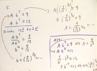
We can solve the third system by dividing the first equation by the second in order to eliminate the variable A. We obtain b^4 = (9/12), which we can easily solve for b. Note that the solution should be b = +-(9/12)^(1/4) = +-.930604859. We can then substitute our value of b back into either of the original equations (the first in the example shown below), obtaining an equation in A alone. We easily solve this equation for A. The solutions are a = 14.88967774 , b = 0.930604859 and, a = -14.88967774 , b = -0.9306048591.
An alternative solution of the third system would be to solve the first equation for A and substitute the value into the second, as shown in the lower right-hand quarter of the figure below. We obtain an equation for b, which gives us the same solution as our previous equation for b. We then proceed in the same manner as before.
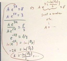
The fourth system of equations, as shown in the second figure below, can also the solved by dividing the first equation by the second. However, since the variable k is in the exponent, our solution of the resulting equation e^-(2k) = 8/3 will require the use of logarithms. We proceed to take a natural log of both sides, obtaining an equation we can easily solve for k, obtaining k = -0.4904146265. We then substitute this value for k into the first of the original equations, obtaining an equation in A alone. The intimidating exponential term in this equation is just a number which, following the order of operations, we can easily evaluate on calculator. So we will easily obtain the value of A. We get A = 34.83718745.
6. Solving Exponential Equations
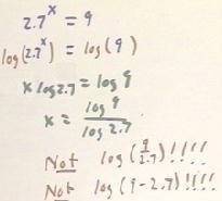
The first equation is easily solved by taking the logarithm of both sides. Using the laws of logarithms we obtain x log(2.7) = log 9. Calculating our solution x = log 9 / log(2.7) we must be careful not to succumb to the temptation to do log(9/2.7), which by the laws of logarithms is log 9 - log 2.7, or in confusion with this law trying to do log(9 - 2.7), which has very little to do with anything. Evaluate log 9, evaluate log 2.7, and divide the two. We obtain x = 2.212152630.
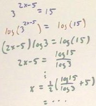
We use the same strategy in solving the second equation. We quickly obtain 2x - 5 = log 15 / log(3). Then we add 5 to both sides and multiply by 1/2 to obtain our final solution, which we easily evaluate with a calculator, obtaining x = 3.732486739.
Similar strategies are used with the third fourth equations. The solution to the third is x = -4.276989408 and the solution to the fourth is x = 2.523718997.
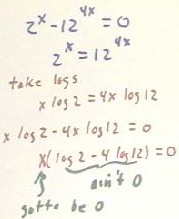
We cannot simply take the log of both sides of the last equation, since there is no way to simplify an expression of the form log(a-b) (check out the laws of logarithms to be sure you understand this). However, we can add 12 ^ (4x) to both sides and then take logs. When we do we obtain an equation with a factor x on both sides. We rearrange the equation so both of these factors are on the same side, then factor out x. Since the factor log 2 - 4 log(12) is not 0, and since the product of the two factors is 0, the other factor, namely x, must be 0.
7. Solving Logarithmic Equations
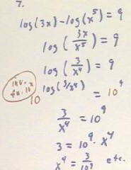
We solve the first equation using the laws of logarithms to combine the two terms of the left-hand side into the expression log(3 / x^4). We can then use the inverse function 10^z to bring the x expression out of the exponent. We exponentiate both sides, as indicated in the fourth line, and obtain the equation 3 / x^4 = 10^9. After multiplying both sides by the denominator x^4, we obtain an equation we can easily solve for x. Our solution is x = +- (3/10^9)^(1/4), which simplifies to x = +- 0.007400828044
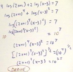
We use a similar strategy on the second equation. Before combining the two log terms into 1,we must use the property that a log b = log(b^a), as in the second line. We then use the property that log a + log b = log(ab) to obtain the expression in the third line. We apply the inverse function to both sides in the fourth line. In the fifth line we realized we are in trouble. We try to get out of trouble by taking the 1/2 power of both sides in the sixth line, but after simplifying to obtain the seventh line we realized we have a cubic polynomial. While there is an algorithm to solve cubic polynomials, it is fairly painful so we resign ourselves to DERIVE.
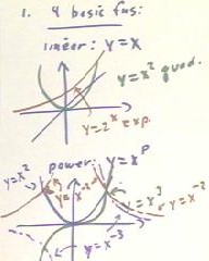
We obtain x = 3.513861421.1. The four basic functions
Sketch graphs of the four basic functions, clearly indicating the key graphing points. For power functions sketch graphs of the p= +-2 and +-3 functions.
We cannot represent the power functions by one graph, since different powers have graphs with different characteristics. However, if we graph the x^2, x^3, x^-2 and x^-3 functions, using the points x = -2, -1, -1/2, 0, 1/2, 1, 2, we see the pattern that emerges for positive and negative powers of greater magnitude. We note how the behavior at x = 1/2 shows us that the positive-power graphs will flatten out near the origin as the power increases. We note how every one of these graphs will pass through the point (1,1), while the even powers will pass through (-1,1) and the out powers through (-1,-1). We see that even powers are even functions, symmetric with respect to the y axis, while the odd powers are odd functions, antisymmetric with respect to the y axis and symmetric with respect to the origin.
2. Inverse functions
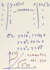
Give several examples of pairs of inverse functions. Explain how a table of y vs. x values for function which has an inverse is used to make the table for the y vs. x values of the inverse function, and how to construct a graph of the inverse of a function from the graph of the function. Explain also to determine from the graph of a function when the function does not have an inverse.
As depicted in the figure below we obtain a partial table for the inverse of a function y = f(x) by reversing the columns of a y vs. x table. The table we obtain it is the table of y = f^-1 (x) vs. x.
Examples of inverse functions include
When we graph a function on the same set of coordinate axes as its inverse, the two functions will be symmetric about the line y = x. Corresponding points of the tables can be joined by line segments which meet the y = x line at a perpendicular, with the corresponding points at equal distances from the y = x line.
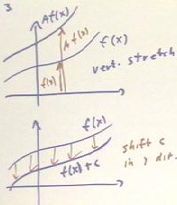
3. Stretching and shifting transformations
For each of the four basic functions, show the family A f(x), f(x-h) and f(x) + c; explain how to obtain the function A f(x-h) + c, and show one good illustrative example of this function.
These transformations are amply covered in recent class notes. We simply note that
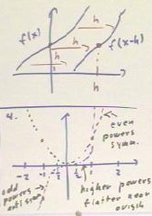
4. Power functions
Sketch graphs of the p = +-2 and p = +-3 power functions, clearly showing their behavior at the key points and indicating how this behavior will continue for greater magnitudes of p.
The graphs of y = x^2 and y = x^3 are shown below. We see clearly some of the behaviors described in #1 above.
5. Polynomial Functions
For a given degree n, indicate all possible numbers of zeros for a polynomial of that degree. Show every possible variation in the behavior of the function at its zeros and sketch a graph depicting each possibility.
Polynomial function have been covered thoroughly and recently. Refer to class notes and handouts.
6. Composite Functions
Express each of the following is a composite f(g(x)) of the four fundamental function families:
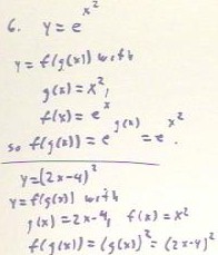
The function y = e^(x^2) is of the form y = f(g(x)), with g(x) = x^2 and f(x) = e^x. We see this because straightforward substitution, using function notation, gives us f(g(x)) = e^(g(x)) = e^(x^2).
Similarly we see that y = (2x - 4)^2 is of the same form, with g(x) = 2x - 4 and f(x) = x^2. Use substitution and function notation to convince yourself that for these functions, f(g(x)) = (2x - 4) ^ 2.
y = 2 e^x + 4 is a composite f(g(x)) with f(x) = 2x+4 and g(x) = e^x.
y = (e^x)^2 is a composite f(g(x)) of f(x) = x^2 and g(x) = e^x.
y = 6 (e^x)^2 is a composite f(g(x)) of f(x) = 6 x^2 and g(x) = e^x.
y = 12 (e^x)^-4 is a composite f(g(x)) of f(x) = 12 x^-4 and g(x) = e^x.
7. Constant Multiples, Sums and Differences of Functions
For each of the following function pairs graphically construct a graph of f(x) + g(x), f(x) - g(x), 2 f(x) and -1/3 g(x).
f(x) = x^2 - 3x - 2, g(x) = 2x - 6, -4 < x < 4
8. Products of Functions
For each of the following function pairs graphically construct a graph of f(x) * g(x) and f(x) / g(x).
This topic has been covered in recent class notes and handouts.