class 050902
My Question is... On our exercies you assigned today, Aug. 31... I do not
understand the
directions... Do we use the same formula we used for the water depth expirment?
And do we
only do Data set 1 and 2 or should we read ahead of that?
Good question. This one was answered in an email sent to everyone in the
class.
Hey dave, I'm not confused about anything but I would like to know when solving
for c after
you have unknowns a and b does it matter which equation you solve it in?
If you've solved correctly for a and b, then you'll get the same thing no
matter which
equation you use.
Similarly if you've eliminated c, then eliminated b from the two resulting
equations, and
then finally solved for a, it doesn't matter which of the two equations you
substitute a
into, you'll get the same result for b.
Once you've used your values of a and b to get c from one of the original
equations, you
should then substitute your a, b and c into another one of the original
equations to check
your work.
Another way of checking, of course, is to get your model y = a t^2 + b t + c and
then to
substitue your chosen t values. Each of your chosen t values should give you the
corresponding y value.
What exactly do you mean when you say the word model, because you sometimes
refer to a graph
or a mathimatical equation, and when you say model it doesn't specify which one
you want, a
graph or an equation?
The model is the function, which is represented by both the graph and the
model.
The function can usually be expressed as a graph or an equation.
For example the depth vs. clock time function might be y = f(t) = .41 t^2 - 3.74
t + 94.
The equation is y = .41 t^2 - 3.74 t + 94, and the graph represents this
function.
The graph represents the equation, and the equation represents the graph, so the
two are
actually identical. The equation is generally more accurate than the graph, but
within
limits of accuracy the equation and the graph tell you exactly the same thing.
What they
both represent is the function.
If T=.23L^.48 and that is a constant then can those numbers always be put into
any equation,
like T=A*L^p?
y = A x^p is the general form of a power function y of the independent
variable x.
Our pendulum period vs. length function uses variables T and L instead of y and
x.
So T = A * L^p is the general form of a power function T of the independent
variable L.
Knowing that the pendulum period should be a power function of its length, we
would then
know to use the form T = A * L^p. If we know the values of T at two different
values of L,
we can then substitute each pair of values into the form to get an equation in
the
parameters A and p (see notes from late in the first week for specific examples
of this).
Once we have two equations in A and p, we can solve them for A and p.
Having obtained our values of A and p, we then plug them into the form T = A *
L^p, giving
us our mathematical model of period T as a function of length L.
The model we got from our observations in class (again see notes from week 1) is
pretty
close to T = .23 L^.48.
The ideal model given by physics is T = .20 L^.50. So we did pretty well.
My question is... When you say that we need to memorize the above outline of the
model, are
you talking about model part C(Validate and use the model)? or model part
A(Obtain and
represent Date), B (Obtain a Model), & C(Validate and use the model)?
This is the outline you are expected to memorize, and which will be used
throughout the course.
Summary of Modeling Process, Version 3
A. Obtain and Represent Data
A1. Orient
A2. Observe
A3. Organize Data
A4. Graph
B. Obtain a Model
B1. Postulate
B2. Select Representative Points
B3. Obtain an equation for each selected point
B4. Solve the system of equations
B5. Substitute parameters
C. Validate and Use the Model
C1. Graph the model
C2. Quantify the comparison
C3. Pose and answer questions
C4. Do the science: relate the mathematics to the real world.
To Be Memorized
The above outline of the model is to be memorized. At any time during the
course, on any test or quiz, you might be asked to write down this model and
illustrate the meaning of one or more of the steps.
This outline will be more or less followed throughout the course.
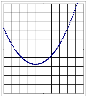
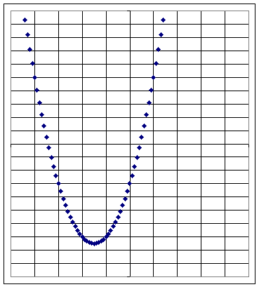
What is the vertex exactly and how exactly do we find it?
We will see more about this in the last of the worksheets in Wednesday's
handout, the Assignment 3 worksheet "Properties of Quadratic Functions".
A brief answer is:
y = a t^2 + b t + c is the equation of a parabola. The graph of this equation
has the shape of a parabola (a parabola is a curve with the property that every
point of the curve lies at the same distance from its focus and directrix, but
the details of that definition and how it is related to the equation given here
is a second-semester topic).
The parabola is symmetric about a vertical line. The point where the parabola
intersects this vertical line is called the vertex. It is either the high or the
low point of the parabola, depending on whether the parabola opens upward or
downward.
The axis of symmetry is the line t = - b / ( 2 a), where a and b are the
coefficients of t^2 and t.
You can find the y coordinate of the vertex by substituting this t value into
the equation of the parabola.
basic precalculus functions with parameters.xls
For the first problem on your homework for today:
At clock time 46 sec, t = 46. We plug in 46.
If our function is y = f(t) = .01 t^2 - 2 t + 100 we get
y = f(46) = .01*46^2 - 2 * 46 + 100 = etc.
Water depth is 14 cm when y = 14. Substitute 14 into the model to get
14 = .01 t^2 - 2 t + 100.
quad formula applies to y = a t^2 + b t + c, when y = 0.
In our equation y isn't 0. What are we gonna do?
If we subtract 14 from both sides we get
.01 t^2 - 2 t + 86 = 0.
Now we can apply the quadratic formula, with a = .01, b = -2 and c = 86.
For the second problem, using Data Set 1 on grade average vs. percent of classes reviewd
Assignment 3
q_a_ Assignment 3.
See also Class Notes #03
Properties of Quadratic Functions
note that the DOS program QUADEQ provides useful practice; use it if practice is required
Optional Exercises for Practice: Graphs of selected parabolas (a series of DOS-based exercises)
Introduction to Matrices (Beginning Summer 01): Assignment will be posted prior to due date.
Most Basic Properties of Linear, Quadratic and Exponential Functions: Practice until you can instantly and accurately sketch these graphs.
When you have completed the entire assignment run the Query program.
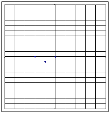
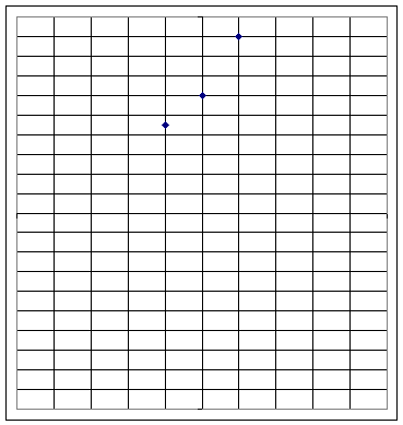
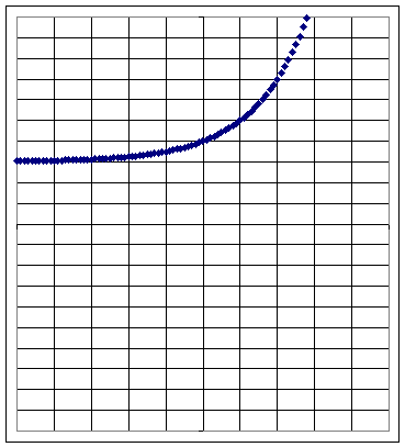
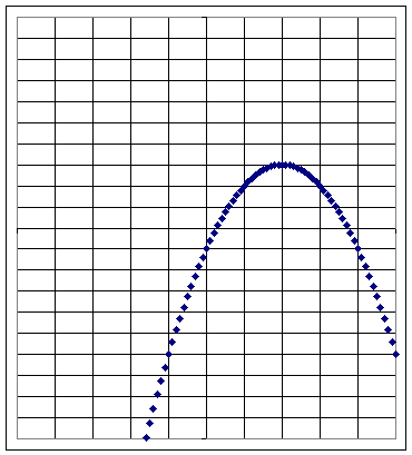
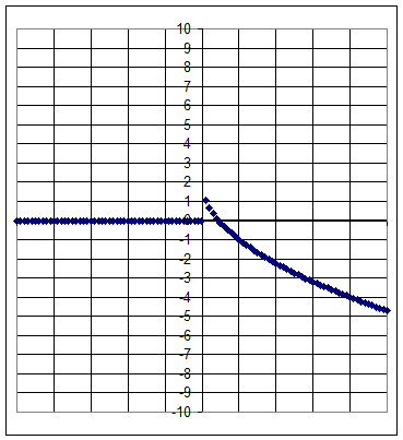
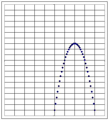
Graph 1
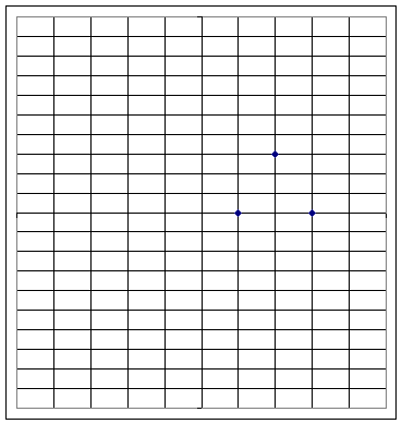
Graph 2
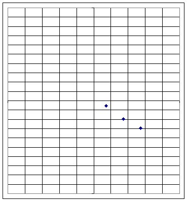
Graph 3
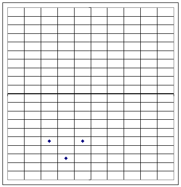
Graph 4
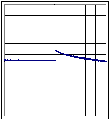
Graph 1a
Graph 2a
Graph 3a
Graph 4a
Graph 1b
Graph 2b
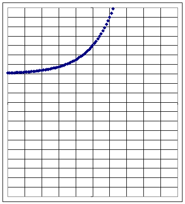
Graph 3b
Graph 4b
Graph 5b
Graph 6b
Graph 7b
Graph 8b
Graph 9b